# Optional: run once if you want to use Levene's test
# install.packages("car")F-Test and ANOVA
C5025HF
Hands‑on: One‑way ANOVA in R
We’ll create a small dataset with one numeric response (yield) and one factor (fert).
fert <- data.frame(
  yield = c(20, 22, 19, 21,
            34, 35, 36, 34,
            27, 28, 29, 28),
  fert = factor(rep(c("A","B","C"), each = 4))
)
Take a quick look:
head(fert) yield fert
1 20 A
2 22 A
3 19 A
4 21 A
5 34 B
6 35 Bsummary(fert) yield fert
Min. :19.00 A:4
1st Qu.:21.75 B:4
Median :28.00 C:4
Mean :27.75
3rd Qu.:34.00
Max. :36.00 table(fert$fert)
A B C
4 4 4
Optional: visualise group differences before modelling.
boxplot(yield ~ fert, data = fert,
        xlab = "Fertiliser", ylab = "Yield",
        col = c("#8dd3c7","#ffffb3","#bebada"))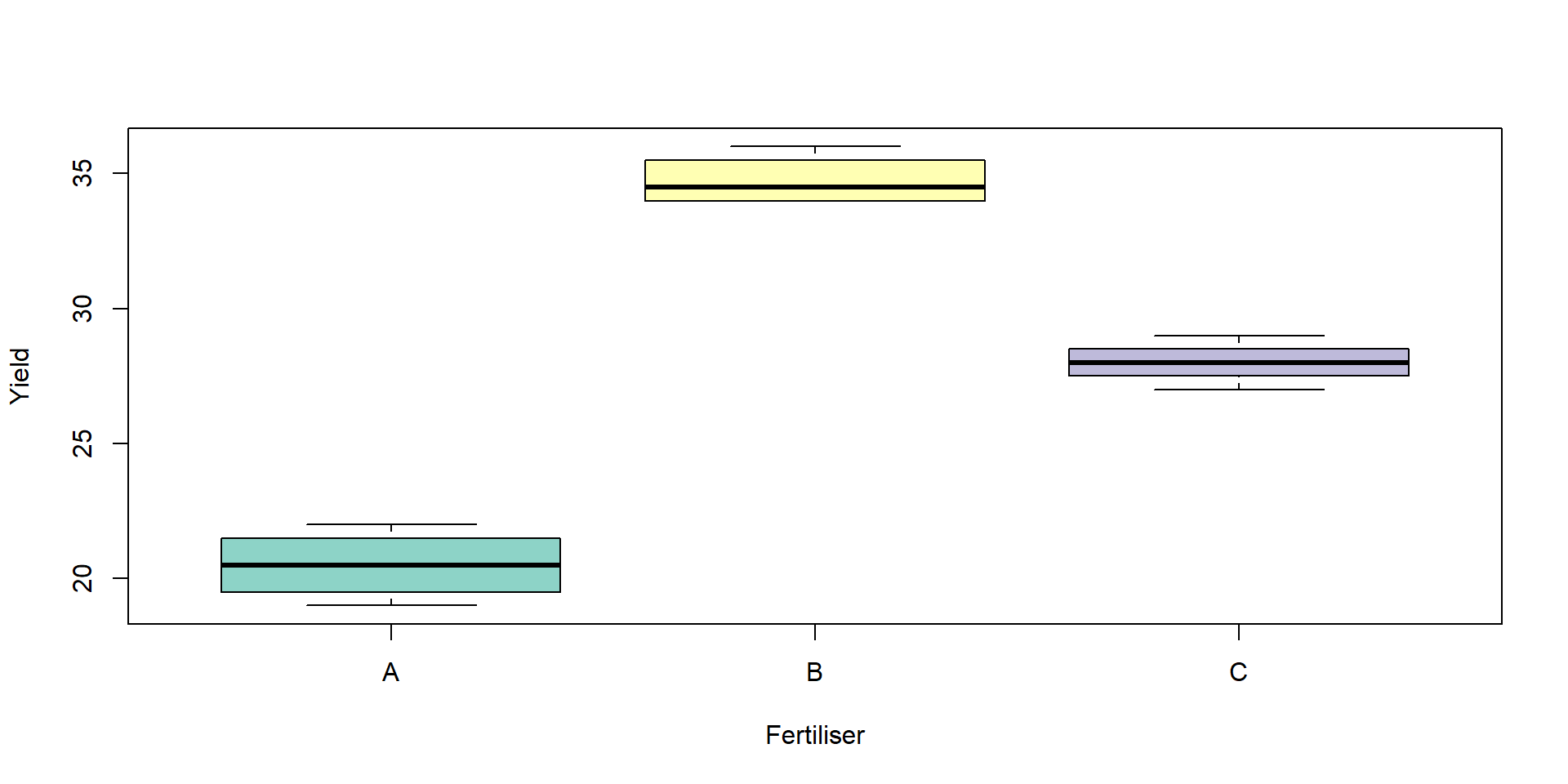
Fit the ANOVA model and view the ANOVA table:
fit <- aov(yield ~ fert, data = fert)
summary(fit)
Df Sum Sq Mean Sq F value Pr(>F)
fert 2 406.5 203.25 187.6 4.61e-08 ***
Residuals 9 9.7 1.08
---
Signif. codes: 0 '***' 0.001 '**' 0.01 '*' 0.05 '.' 0.1 ' ' 1How to read the table:
Df: degrees of freedom (treatment and residual)
Sum Sq: \(SS_B\) and \(SS_W\)
Mean Sq: \(MS_B\) and \(MS_W\)
F value: the test statistic \(F = \frac{\text{MS}_B}{\text{MS}_W}\)
Pr(>F): the p‑value (small p suggests at least one mean differs)
Manual ANOVA (by hand) and verification
Let’s compute the ANOVA components directly and confirm they match aov():
# Group means and counts
group_means <- tapply(fert$yield, fert$fert, mean)
group_counts <- table(fert$fert)
grand_mean <- mean(fert$yield)

# Between-groups sum of squares (SSB)
SSB <- sum(group_counts * (group_means - grand_mean)^2)

# Within-groups sum of squares (SSW)
SSW <- sum(unlist(tapply(fert$yield, fert$fert, function(v) sum((v - mean(v))^2))))

# Degrees of freedom
k <- length(group_means)
N <- nrow(fert)
df_between <- k - 1
df_within  <- N - k

# Mean squares and F
MSB <- SSB / df_between
MSW <- SSW / df_within
F_manual <- MSB / MSW

# Assemble a manual ANOVA table
anova_manual <- data.frame(
  Source = c("fert", "Residuals"),
  Df     = c(df_between, df_within),
  `Sum Sq`= c(SSB, SSW),
  `Mean Sq`= c(MSB, MSW),
  check.names = FALSE
)
anova_manual
Source Df Sum Sq Mean Sq
1 fert 2 406.50 203.250000
2 Residuals 9 9.75 1.083333F_manual[1] 187.6154# Compare with aov()
anova(aov(yield ~ fert, data = fert))Analysis of Variance Table
Response: yield
Df Sum Sq Mean Sq F value Pr(>F)
fert 2 406.50 203.250 187.62 4.607e-08 ***
Residuals 9 9.75 1.083
---
Signif. codes: 0 '***' 0.001 '**' 0.01 '*' 0.05 '.' 0.1 ' ' 1You should see identical sums of squares, degrees of freedom, mean squares, and F.
Assumptions you should check
ANOVA relies on:
Independence of observations (this is a design issue).
Approximately normal residuals.
Homogeneity of variances across groups.
The standard diagnostic plots are a good start:
par(mfrow = c(2,2))
plot(fit)par(mfrow = c(1,1))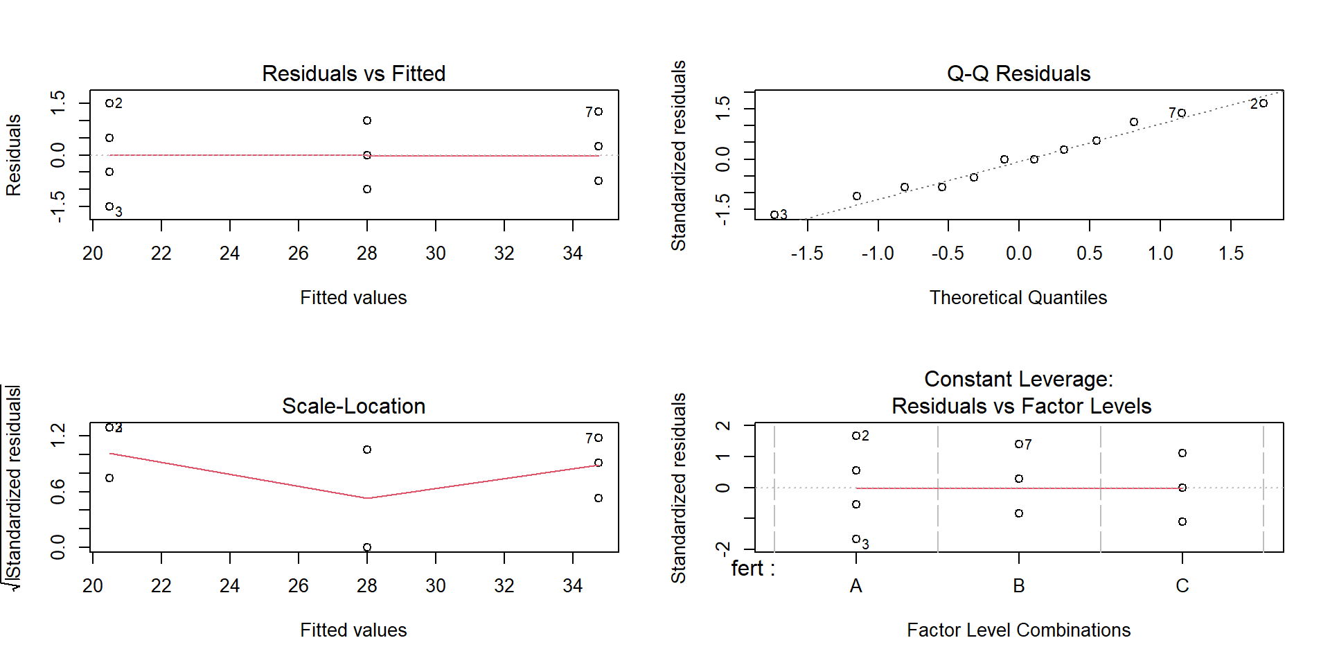
What to look for:
Residuals vs Fitted: no strong patterns or funnels.
Normal Q‑Q: points near a straight line.
Formal checks (optional and context‑dependent):
# Normality of residuals
shapiro.test(residuals(fit))
    Shapiro-Wilk normality test

data:  residuals(fit)
W = 0.96598, p-value = 0.8645
# Homogeneity of variances (choose one)
bartlett.test(yield ~ fert, data = fert) # Bartlett's test (sensitive to non‑normality)
    Bartlett test of homogeneity of variances

data:  yield by fert
Bartlett's K-squared = 0.57949, df = 2, p-value = 0.7485
# If you installed 'car':
# car::leveneTest(yield ~ fert, data = fert) # Levene's test (more robust)If assumptions look poor: consider transforming the response (e.g., log), using a robust method, or revisiting the design/measurement process.
Interpreting the Q‑Q plot (in detail)
First, plot the residuals explicitly so you can inspect their shape.
res <- residuals(fit)
par(mfrow = c(1,2))
qqnorm(res, main = "Normal Q-Q Plot of Residuals")
qqline(res, col = "red", lwd = 2)
hist(res, breaks = 10, col = "gray90", main = "Histogram of Residuals",
xlab = "Residual")par(mfrow = c(1,1))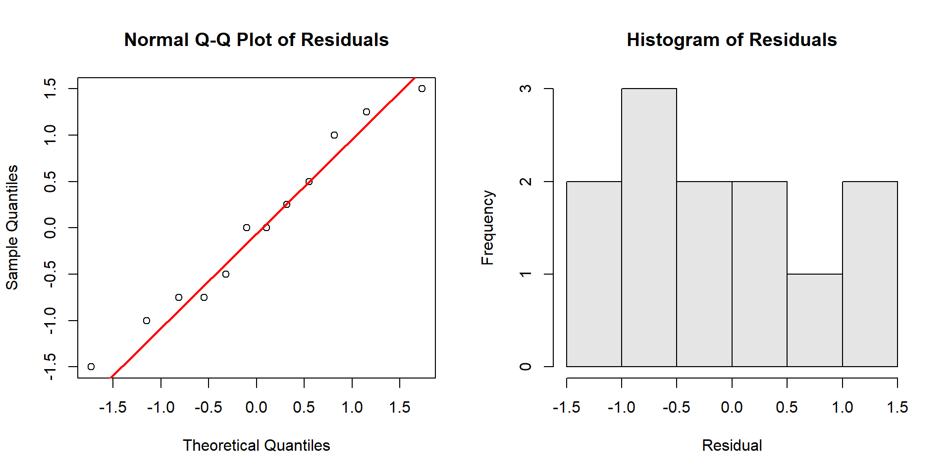
How to read the Q‑Q plot:
- Points close to the straight line → residuals are approximately normal.
- S‑shaped curve (points above the line on the left and below on the right, or vice versa) → skewness.
- Points that bow away at both ends → heavy tails (more extreme residuals than normal).
- Points that stay close in the middle but diverge strongly at ends → tail problems that can affect small‑sample inference.
What to do:
Minor deviations are usually fine; focus on large, systematic patterns.
Consider transformations (e.g., log) for right‑skewed positive data, or a different model if deviations reflect design issues.
Which means differ? Post‑hoc comparisons
ANOVA tells you there is a difference somewhere. To find where, use multiple comparisons that control familywise error.
Tukey’s Honest Significant Difference (HSD):
TukeyHSD(fit) Tukey multiple comparisons of means
95% family-wise confidence level
Fit: aov(formula = yield ~ fert, data = fert)
$fert
diff lwr upr p adj
B-A 14.25 12.19514 16.30486 0.00e+00
C-A 7.50 5.44514 9.55486 8.20e-06
C-B -6.75 -8.80486 -4.69514 1.95e-05You can also visualise the Tukey intervals:
plot(TukeyHSD(fit))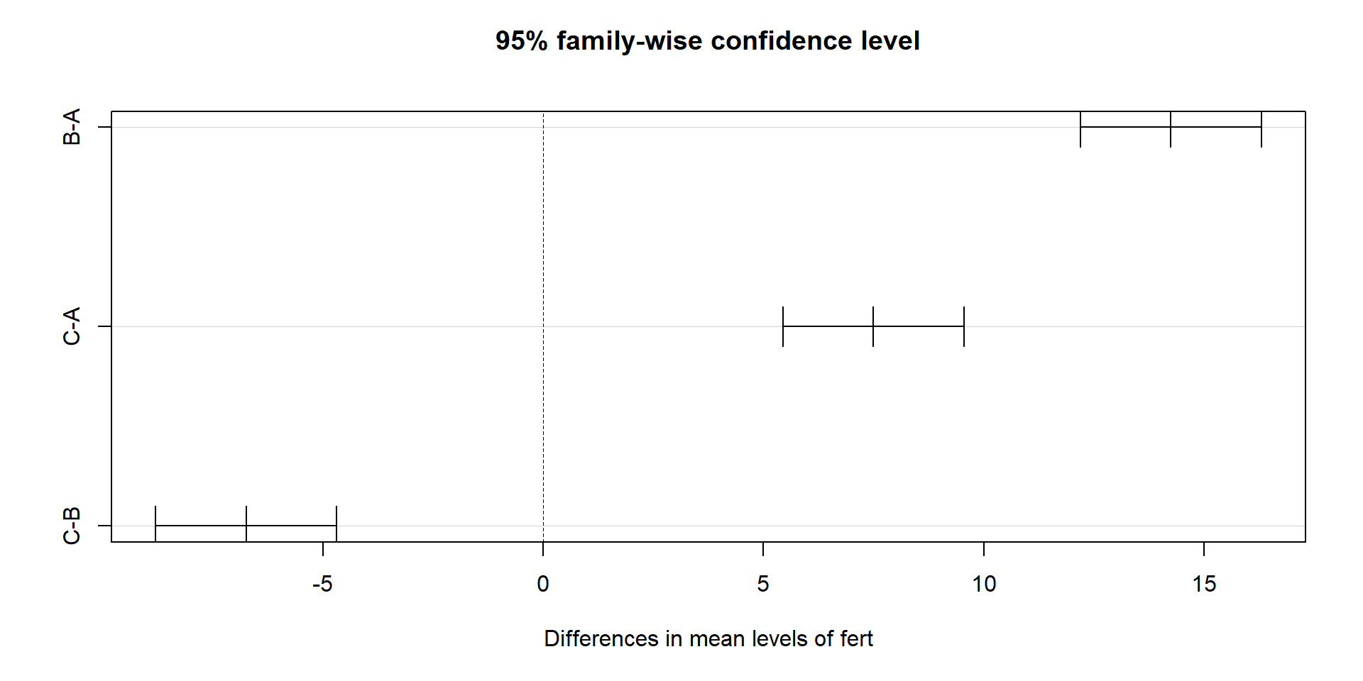
Pairwise t‑tests with p‑value adjustment (alternative approach):
pairwise.t.test(fert$yield, fert$fert, p.adjust.method = "bonferroni")
    Pairwise comparisons using t tests with pooled SD

data:  fert$yield and fert$fert

  A       B
B 3.6e-08 -
C 9.2e-06 2.2e-05

P value adjustment method: bonferroni
How to interpret:
Each pair shows a difference in means, a confidence interval (Tukey), and an adjusted p‑value.
If a confidence interval does not include 0, or the adjusted p‑value is small, that pair differs.
ANCOVA: ANOVA with a covariate
Why you need it:
Sometimes groups differ partly because of a continuous baseline variable (e.g., initial size, starting weight, pre‑test score).
ANCOVA adjusts group comparisons for that covariate, improving precision and providing “fair” comparisons at the same covariate level.
Conceptually, you fit parallel regression lines with a common slope across groups and compare their intercepts (adjusted means).
set.seed(2)
n_per <- 12
ancova <- data.frame(
  fert = factor(rep(c("A","B","C"), each = n_per)),
  size0 = rnorm(3 * n_per, mean = 10, sd = 2)
)
# True treatment effect and slope
beta0 <- 5; slope <- 0.8
trt_effect <- c(A = 0, B = 1.2, C = 2.0)
ancova$yield <- with(ancova, beta0 + trt_effect[fert] + slope * size0 + rnorm(nrow(ancova), 0, 1))

# Parallel slopes model (no interaction)
fit_ancova <- aov(yield ~ fert + size0, data = ancova)
summary(fit_ancova)
Df Sum Sq Mean Sq F value Pr(>F)
fert 2 17.91 8.95 6.299 0.00494 **
size0 1 76.56 76.56 53.858 2.41e-08 ***
Residuals 32 45.49 1.42
---
Signif. codes: 0 '***' 0.001 '**' 0.01 '*' 0.05 '.' 0.1 ' ' 1# Optional: test for non-parallel slopes
fit_ancova_int <- aov(yield ~ fert * size0, data = ancova)
anova(fit_ancova, fit_ancova_int)Analysis of Variance Table
Model 1: yield ~ fert + size0
Model 2: yield ~ fert * size0
Res.Df RSS Df Sum of Sq F Pr(>F)
1 32 45.489
2 30 42.782 2 2.7065 0.9489 0.3985Visualising parallel slopes (from the ANCOVA fit):
lm_ancova <- lm(yield ~ fert + size0, data = ancova)
cols <- c(A = "#1b9e77", B = "#d95f02", C = "#7570b3")
plot(yield ~ size0, data = ancova, col = cols[fert], pch = 19,
     main = "ANCOVA: parallel slopes by treatment", xlab = "Baseline size (size0)", ylab = "Yield")
legend("topleft", legend = levels(ancova$fert), col = cols, pch = 19, bty = "n")
slope_hat <- coef(lm_ancova)["size0"]
intercepts <- c(
  A = coef(lm_ancova)["(Intercept)"],
  B = coef(lm_ancova)["(Intercept)"] + coef(lm_ancova)["fertB"],
  C = coef(lm_ancova)["(Intercept)"] + coef(lm_ancova)["fertC"]
)
xg <- seq(min(ancova$size0), max(ancova$size0), length.out = 100)
for (g in names(intercepts)) {
  lines(xg, intercepts[g] + slope_hat * xg, col = cols[g], lwd = 2)
}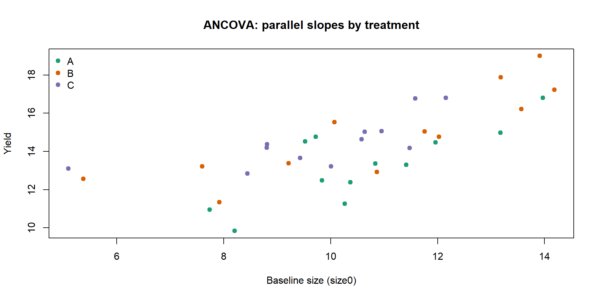
Interpretation:
size0reduces residual variation by explaining baseline differences;ferttests adjusted group shifts.If the
fert:size0interaction is not significant, parallel slopes are a good summary; if significant, the treatment effect depends on the covariate.
Assumptions (in addition to ANOVA’s):
Linearity between the covariate and the response within groups.
Homogeneous slopes across groups (if using the parallel slopes model).
Covariate measured without substantial error and not affected by treatment (pre‑treatment).
MANOVA: multiple responses
Why you need it:
Many experiments record multiple, correlated outcomes (e.g., plant height and leaf area; multiple biochemical markers).
Running separate ANOVAs inflates the familywise error rate and ignores correlation structure.
MANOVA tests for differences in the multivariate mean vector across groups, leveraging correlation to increase power and control Type I error.
What it provides:
A single global test (e.g., Wilks’ Lambda) for whether groups differ on the joint set of responses.
If significant, you can follow up with univariate ANOVAs and multivariate visualisation to understand where differences arise.
set.seed(3)
m <- data.frame(
  fert = factor(rep(c("A","B","C"), each = 15))
)
mu <- cbind(A = c(0, 0), B = c(0.8, 0.4), C = c(1.2, 0.9))
Sigma <- matrix(c(1.0, 0.5, 0.5, 1.2), 2, 2)  # positive correlation
# If MASS is not available, fall back to independent normals
if (!requireNamespace("MASS", quietly = TRUE)) {
  set.seed(3)
  y1 <- c(rnorm(15, mu[1, "A"], sqrt(Sigma[1,1])),
          rnorm(15, mu[1, "B"], sqrt(Sigma[1,1])),
          rnorm(15, mu[1, "C"], sqrt(Sigma[1,1])))
  y2 <- c(rnorm(15, mu[2, "A"], sqrt(Sigma[2,2])),
          rnorm(15, mu[2, "B"], sqrt(Sigma[2,2])),
          rnorm(15, mu[2, "C"], sqrt(Sigma[2,2])))
} else {
  set.seed(3)
  yA <- MASS::mvrnorm(15, mu = mu[, "A"], Sigma = Sigma)
  yB <- MASS::mvrnorm(15, mu = mu[, "B"], Sigma = Sigma)
  yC <- MASS::mvrnorm(15, mu = mu[, "C"], Sigma = Sigma)
  y1 <- c(yA[,1], yB[,1], yC[,1])
  y2 <- c(yA[,2], yB[,2], yC[,2])
}
m$y1 <- y1
m$y2 <- y2

fit_man <- manova(cbind(y1, y2) ~ fert, data = m)
summary(fit_man, test = "Wilks")
Df Wilks approx F num Df den Df Pr(>F)
fert 2 0.4634 9.6144 4 82 2e-06 ***
Residuals 42
---
Signif. codes: 0 '***' 0.001 '**' 0.01 '*' 0.05 '.' 0.1 ' ' 1Quick visual check of separation:
cols <- c(A = "#1b9e77", B = "#d95f02", C = "#7570b3")
plot(m$y1, m$y2, col = cols[m$fert], pch = 19,
     xlab = "y1", ylab = "y2", main = "Scatter of responses by treatment")
legend("topleft", legend = levels(m$fert), col = cols, pch = 19, bty = "n")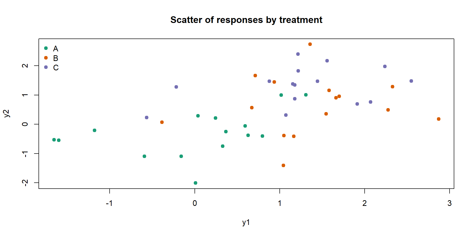
Interpretation and assumptions:
A significant Wilks’ test suggests group centroids differ in the 2D space.
Assumptions: multivariate normality of residuals, equal covariance matrices across groups (Box’s M), and independence. With small samples, be cautious.
Follow‑ups: inspect univariate ANOVAs and confidence ellipses (or discriminant analysis) to interpret which responses drive the separation.
Repeated measures ANOVA (within‑subjects)
Why you need it:
The same subject (or plot) is measured under multiple conditions or times; repeated measures increase efficiency but violate independence.
Repeated measures ANOVA accounts for within‑subject correlation by modelling subjects as a random block and testing the within‑subject factor.
set.seed(4)
subjects <- factor(1:12)
rm_dat <- expand.grid(subject = subjects, treatment = factor(c("A","B","C")))
# Random subject intercepts
subj_eff <- rnorm(length(subjects), 0, 0.8)
rm_dat$response <- with(rm_dat,
  5 + (treatment == "B")*0.8 + (treatment == "C")*1.5 +
  subj_eff[subject] + rnorm(nrow(rm_dat), 0, 0.5)
)
fit_rm <- aov(response ~ treatment + Error(subject/treatment), data = rm_dat)
summary(fit_rm)
Error: subject
          Df Sum Sq Mean Sq F value Pr(>F)
Residuals 11  18.19   1.654

Error: subject:treatment
          Df Sum Sq Mean Sq F value   Pr(>F)
treatment  2  8.899   4.449      21 7.92e-06 ***
Residuals 22  4.661   0.212
---
Signif. codes:  0 '***' 0.001 '**' 0.01 '*' 0.05 '.' 0.1 ' ' 1
Simple visualisation of subject trajectories:
cols <- rainbow(length(subjects), alpha = 0.5)
plot(1, type = "n", xlim = c(1, length(levels(rm_dat$treatment))), ylim = range(rm_dat$response),
     xaxt = "n", xlab = "Treatment", ylab = "Response", main = "Subject trajectories across treatments")
axis(1, at = 1:length(levels(rm_dat$treatment)), labels = levels(rm_dat$treatment))
for (s in levels(subjects)) {
  ds <- subset(rm_dat, subject == s)
  ord <- order(ds$treatment)
  lines(1:length(ord), ds$response[ord], col = cols[as.integer(s)], lwd = 1.5)
  points(1:length(ord), ds$response[ord], col = cols[as.integer(s)], pch = 19)
}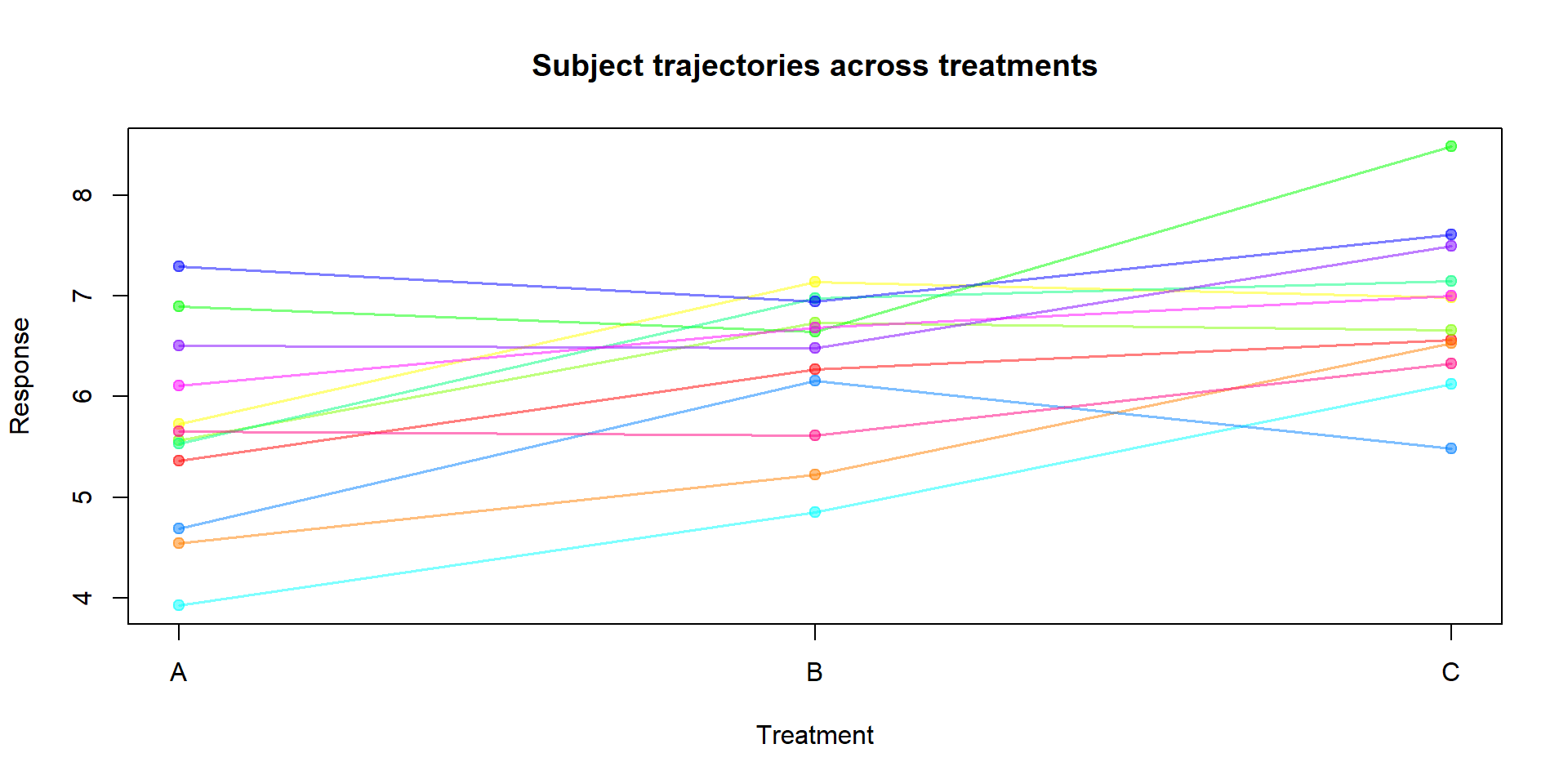
Interpretation and assumptions:
The within‑subject test of
treatmentappears underWithinin theError: subject:treatmentstratum.Sphericity (equal variances of differences between all pairs of levels) is an additional assumption for factors with >2 levels; if violated, corrections (Greenhouse–Geisser, Huynh–Feldt) are used. In more complex designs, consider linear mixed models.