Non-Parametric Statistics

C5025HF

Dr K.J. Mhango

Welcome

What You Will Learn Today

Parametric vs non-parametric intuition
Ranking logic and distribution-free ideas
Mann–Whitney, Wilcoxon, Kruskal–Wallis
Correlations: Spearman & Kendall
Exact tests (Fisher)

1: Why Non‑Parametrics?

When parametric assumptions break

Non-normal data
Skewed distributions
Ordinal measurements
Heterogeneous variances
Small samples
Outliers

Ranking-based thinking: The “Race” Analogy

Instead of looking at exact times (values), look at finishing positions (ranks).

The Intuition: Team A vs Team B (Independent)

Imagine a race between two teams.

Parametric (t-test): Compares the Average Time of Team A vs Team B.
- If one runner in Team A takes 5 hours (outlier), Team A’s average is ruined.
Non-Parametric (Mann-Whitney): Compares the Finishing Positions (Ranks).
- It combines everyone (both teams) into one single lineup from 1st to last.
- Then it looks at where Team A falls vs Team B.
- If that slow runner takes 5 hours or 5 days, they are still just “Last Place”. The rank (last) is the same.

The Intuition: Before vs After (Paired)

Imagine the same runner running twice (Race 1 vs Race 2).

Parametric (Paired t-test): Calculates the improvement (Time 1 - Time 2) for each runner, then averages them.
- One runner improving by 5 hours makes the whole group look vastly improved on average.
Non-Parametric (Wilcoxon Signed-Rank):
- It calculates the change for each runner.
- It ranks these changes by size (ignoring direction). Small change = Rank 1, Huge change = Rank 100.
- Then it asks: “Are the biggest ranks associated with getting faster or getting slower?”
- If one runner improves by 5 hours, they get the highest rank, but they don’t pull the magnitude of the sum to infinity. It caps the influence of the outlier.

Why this is useful

Robust to Outliers: Extreme values don’t pull the results (unlike the mean).
Skew doesn’t matter: We are testing the order, not the bell curve.
Any units work: cm, mm, log-transformed, or “Likert scales” — as long as you can say “A > B”, you can rank.

What the tests actually ask

Mann–Whitney (2 groups): If I pick one random value from Group A and one from Group B, is A likely to be higher than B?
Wilcoxon (Paired): It looks at the change in each pair. Do the big changes tend to be increases or decreases?
- (It ranks the size of the changes, then checks if the positive ranks outweigh the negative ranks).
Kruskal–Wallis (>2 groups): Do some groups systematically rank higher than others?

What to report

Descriptive stats: Medians and Interquartile Ranges (IQR) for each group.
Effect size / Direction: Explain the direction of the difference in plain English.
- Instead of just “p < 0.05”, say: “Species A tends to have higher values than Species B.”
- Optional but good: “The probability that a random value from Group A exceeds Group B is approx X%.”
Visuals: Always include a boxplot or jitter plot to show the spread and overlap.

2: Choosing the Right Test

Cheat Sheet

Design	Parametric	Non-parametric
2 independent groups	t-test	Mann–Whitney
2 paired measures	paired t	Wilcoxon signed-rank
>2 independent groups	ANOVA	Kruskal–Wallis
Correlation	Pearson	Spearman, Kendall
2×2 association	χ² test	Fisher exact

3: t-test Using iris

Goal

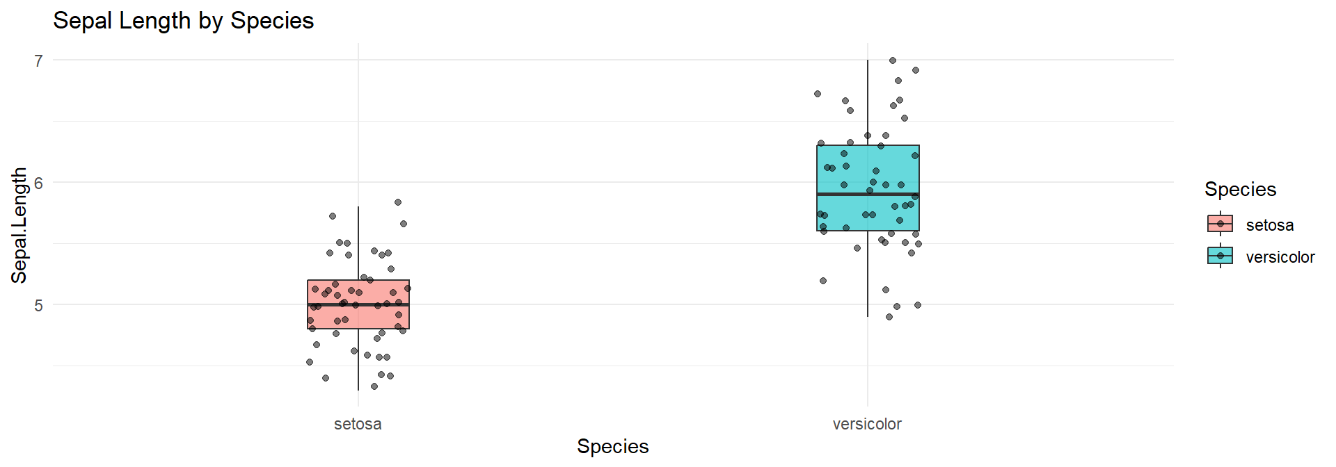
Compare Sepal.Length between two species. We subset to two species for a t-test:

Code

iris2 <- subset(iris, Species %in% c("setosa", "versicolor"))

Visualise

Code

library(ggplot2)
ggplot(iris2, aes(x = Species, y = Sepal.Length, fill = Species)) +
  geom_boxplot(alpha = 0.6,width=0.2) +
  geom_jitter(width = 0.1, alpha = 0.5) +
  theme_minimal() +
  ggtitle("Sepal Length by Species")

Parametric t-test Assumptions

Independence
- Observations must be independent.
- In iris, each flower is a unique specimen → ✔ OK.
Normality of the outcome within each group
- Test with Shapiro–Wilk.

Code

shapiro.test(iris2$Sepal.Length[iris2$Species=="setosa"])


    Shapiro-Wilk normality test

data:  iris2$Sepal.Length[iris2$Species == "setosa"]
W = 0.9777, p-value = 0.4595

Code

shapiro.test(iris2$Sepal.Length[iris2$Species=="versicolor"])


    Shapiro-Wilk normality test

data:  iris2$Sepal.Length[iris2$Species == "versicolor"]
W = 0.97784, p-value = 0.4647

If p < 0.05 in either group, normality is questionable for that group.
- Also use Q–Q plot:

Code

library(ggplot2)
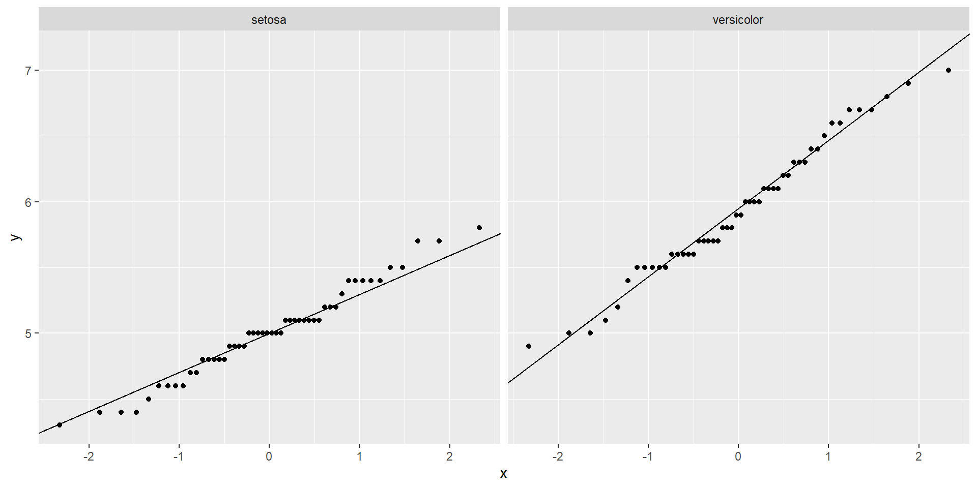
ggplot(iris2, aes(sample = Sepal.Length)) + stat_qq() + stat_qq_line() + facet_wrap(~Species)

Points close to the straight line suggest normality; strong bends or S‑shapes suggest non‑normality.

Homogeneity of variances (Levene test)

Code

library(car)
leveneTest(Sepal.Length ~ Species, data = iris2)

Levene's Test for Homogeneity of Variance (center = median)
      Df F value   Pr(>F)   
group  1  8.1727 0.005196 **
      98                    
---
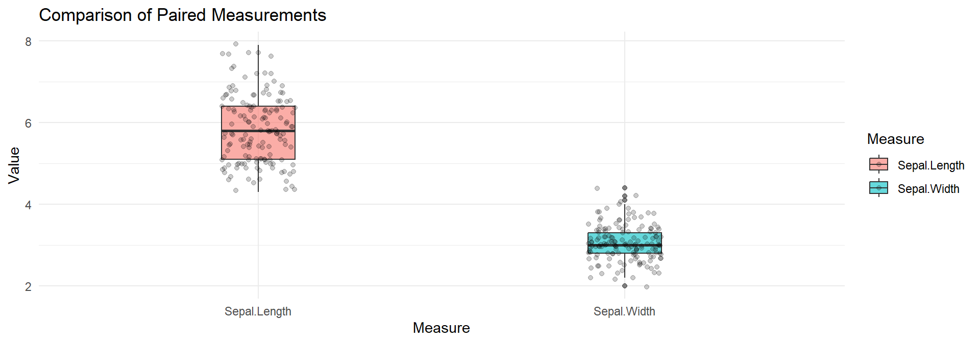
Signif. codes:  0 '***' 0.001 '**' 0.01 '*' 0.05 '.' 0.1 ' ' 1

If p < 0.05, variances differ notably between the two species.

What if assumptions fail?

Non-normality → use Mann–Whitney (Wilcoxon rank-sum).
Heterogeneous variances → Welch t-test OR non-parametric.

Parametric test

Code

t.test(Sepal.Length ~ Species, data = iris2)


    Welch Two Sample t-test

data:  Sepal.Length by Species
t = -10.521, df = 86.538, p-value < 2.2e-16
alternative hypothesis: true difference in means between group setosa and group versicolor is not equal to 0
95 percent confidence interval:
 -1.1057074 -0.7542926
sample estimates:
    mean in group setosa mean in group versicolor 
                   5.006                    5.936

Look for the p-value and the confidence interval; with normality and similar variances, this is appropriate.

Non-parametric alternative (if assumptions break)

Code

wilcox.test(Sepal.Length ~ Species, data = iris2)


    Wilcoxon rank sum test with continuity correction

data:  Sepal.Length by Species
W = 168.5, p-value = 8.346e-14
alternative hypothesis: true location shift is not equal to 0

Use this when data are skewed or have outliers; the p-value tests if one group tends to have higher values.

Example output and interpretation (R)

Code

# Run both to compare

tt_res <- t.test(Sepal.Length ~ Species, data = iris2)
mw_res <- wilcox.test(Sepal.Length ~ Species, data = iris2, exact = FALSE)

tt_res


    Welch Two Sample t-test

data:  Sepal.Length by Species
t = -10.521, df = 86.538, p-value < 2.2e-16
alternative hypothesis: true difference in means between group setosa and group versicolor is not equal to 0
95 percent confidence interval:
 -1.1057074 -0.7542926
sample estimates:
    mean in group setosa mean in group versicolor 
                   5.006                    5.936

Code

mw_res


    Wilcoxon rank sum test with continuity correction

data:  Sepal.Length by Species
W = 168.5, p-value = 8.346e-14
alternative hypothesis: true location shift is not equal to 0

Code

# Print key summaries for the slide
cat("t-test p-value:", format.pval(tt_res$p.value, digits = 3), "\n")

t-test p-value: <2e-16

Code

cat("Mann–Whitney p-value:", format.pval(mw_res$p.value, digits = 3), "\n")

Mann–Whitney p-value: 8.35e-14

Interpret the p-values and medians.
Interpretation: If data look non-normal or have outliers, prefer Mann–Whitney. Report simply, e.g., “Species A tends to have longer sepals than Species B.”

Paired t-test Using iris

Goal

Compare Sepal.Length vs Sepal.Width for the same flowers. Since these measurements come from the same flower, they are paired.

Visualise

Code

# Reshape data to long format for plotting
library(tidyr)
iris_long <- pivot_longer(iris, 
                          cols = c("Sepal.Length", "Sepal.Width"), 
                          names_to = "Measure", 
                          values_to = "Value")

ggplot(iris_long, aes(x = Measure, y = Value, fill = Measure)) +
  geom_boxplot(alpha = 0.6,width=0.2) +
  geom_jitter(width = 0.1, alpha = 0.2) +
  theme_minimal() +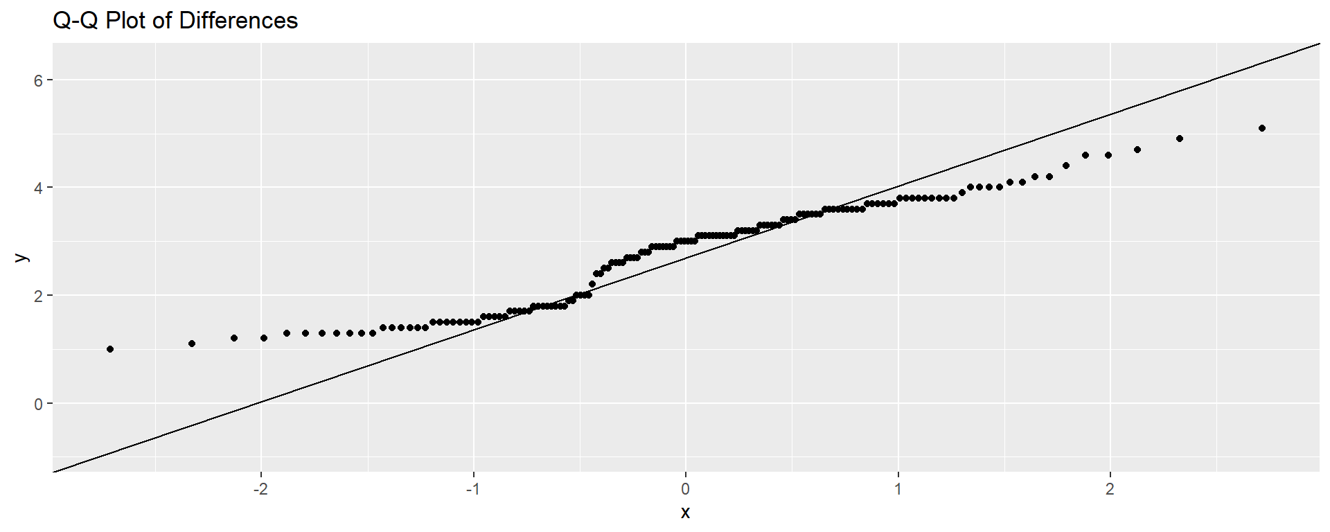
  ggtitle("Comparison of Paired Measurements")

Paired t-test Assumptions

Independence of pairs
- Each flower is independent of others → ✔ OK.
Normality of the differences
- We care about the distribution of \((Sepal.Length - Sepal.Width)\).

Code

diffs <- iris$Sepal.Length - iris$Sepal.Width
shapiro.test(diffs)


    Shapiro-Wilk normality test

data:  diffs
W = 0.94628, p-value = 1.628e-05

If p < 0.05, the differences are not normally distributed.
Check visually:

Code

ggplot(data.frame(diffs), aes(sample = diffs)) + stat_qq() + stat_qq_line() +
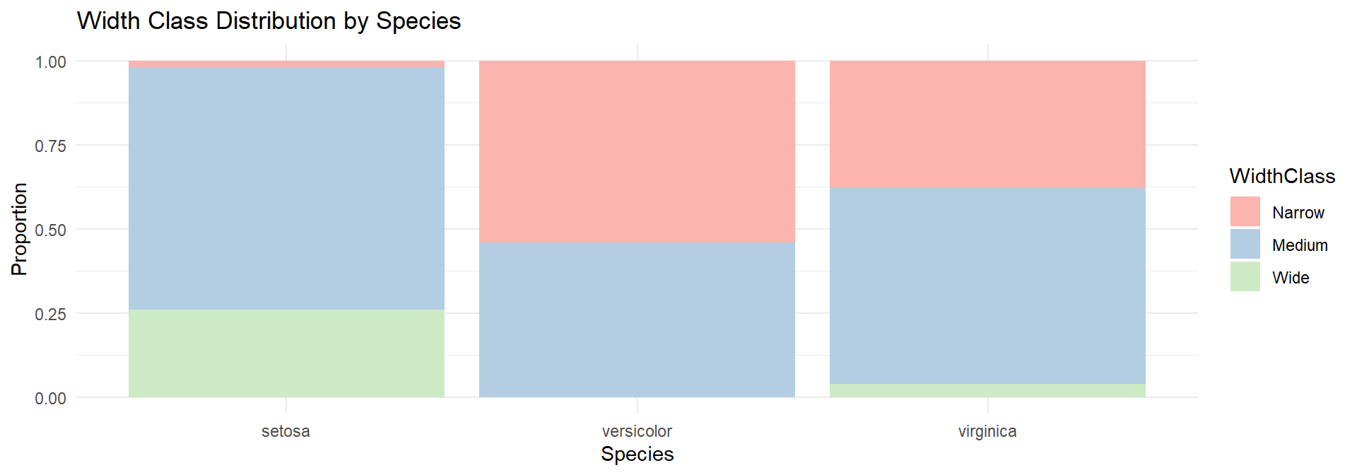
  ggtitle("Q-Q Plot of Differences")

Parametric paired test

Code

t.test(iris$Sepal.Length, iris$Sepal.Width, paired = TRUE)


    Paired t-test

data:  iris$Sepal.Length and iris$Sepal.Width
t = 34.815, df = 149, p-value < 2.2e-16
alternative hypothesis: true mean difference is not equal to 0
95 percent confidence interval:
 2.627874 2.944126
sample estimates:
mean difference 
          2.786

Checks if the mean difference is non-zero.

Non-parametric alternative (if assumptions break)

Wilcoxon Signed-Rank Test

Code

wilcox.test(iris$Sepal.Length, iris$Sepal.Width, paired = TRUE)


    Wilcoxon signed rank test with continuity correction

data:  iris$Sepal.Length and iris$Sepal.Width
V = 11325, p-value < 2.2e-16
alternative hypothesis: true location shift is not equal to 0

Tests if the median difference is non-zero (symmetric assumption) or if the distribution of differences is symmetric around zero.

Example output and interpretation (R)

Code

pair_t <- t.test(iris$Sepal.Length, iris$Sepal.Width, paired = TRUE)
pair_w <- wilcox.test(iris$Sepal.Length, iris$Sepal.Width, paired = TRUE)

pair_t


    Paired t-test

data:  iris$Sepal.Length and iris$Sepal.Width
t = 34.815, df = 149, p-value < 2.2e-16
alternative hypothesis: true mean difference is not equal to 0
95 percent confidence interval:
 2.627874 2.944126
sample estimates:
mean difference 
          2.786

Code

pair_w


    Wilcoxon signed rank test with continuity correction

data:  iris$Sepal.Length and iris$Sepal.Width
V = 11325, p-value < 2.2e-16
alternative hypothesis: true location shift is not equal to 0

Interpretation: “Sepal length is significantly different from sepal width within the same flowers.”

Chi-square Test Using iris

Goal

Test independence between Species and a discretised version of Sepal.Width. We bin Sepal.Width:

Code

iris$WidthClass <- cut(iris$Sepal.Width, breaks = 3, labels = c("Narrow", "Medium", "Wide"))
tab <- table(iris$Species, iris$WidthClass)

Visualise

Code

ggplot(iris, aes(x = Species, fill = WidthClass)) +
  geom_bar(position = "fill") +
  theme_minimal() +
  labs(y = "Proportion", title = "Width Class Distribution by Species") +
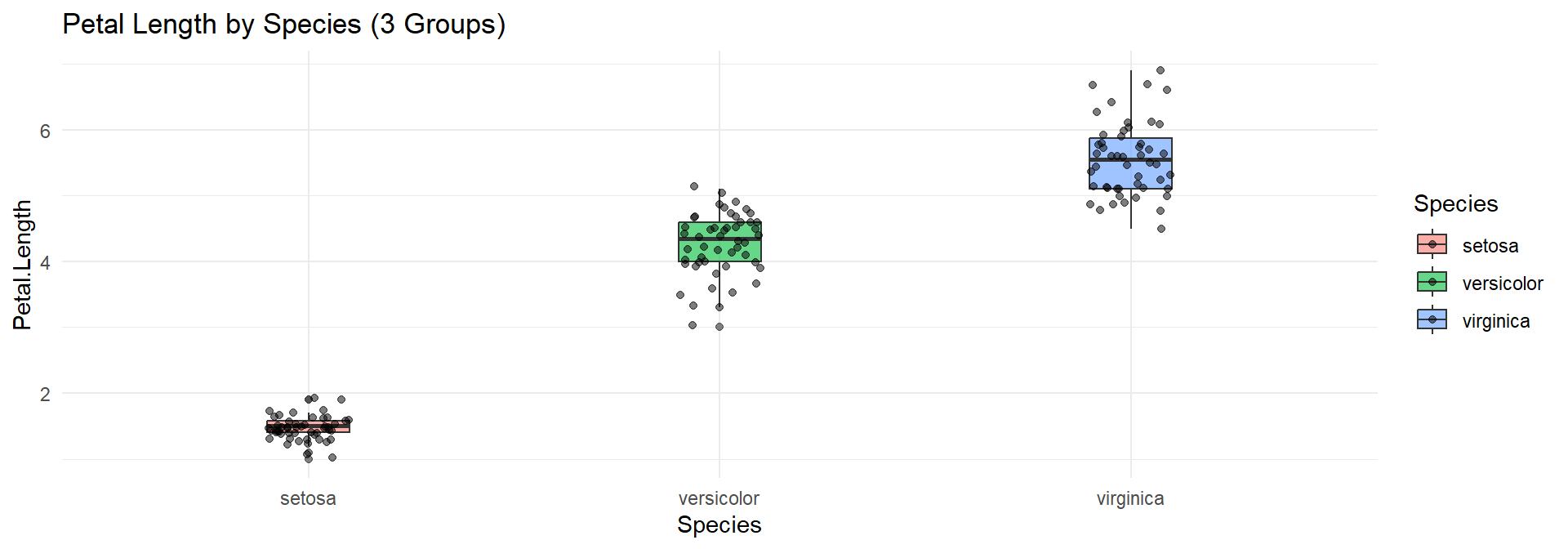
  scale_fill_brewer(palette = "Pastel1")

Chi-square Assumptions

Independence of observations → ✔ OK.
Expected cell counts ≥ 5 in most cells.

Code

chisq.test(tab)$expected

            
               Narrow   Medium Wide
  setosa     15.66667 29.33333    5
  versicolor 15.66667 29.33333    5
  virginica  15.66667 29.33333    5

If expected counts are too small → chi-square invalid. - Scan the table: if any expected cell count is < 5, prefer Fisher’s Exact Test.

Parametric-style categorical test

Code

chisq.test(tab)


    Pearson's Chi-squared test

data:  tab
X-squared = 45.125, df = 4, p-value = 3.746e-09

Chi-square p-value tests association; warnings about small counts mean the test may be unreliable.

Non-parametric alternative when assumptions fail

Fisher’s Exact Test

Works even with small expected cell counts.

Code

fisher.test(tab)


    Fisher's Exact Test for Count Data

data:  tab
p-value = 8.429e-11
alternative hypothesis: two.sided

Fisher’s p-value is reliable even with small expected counts.

Example output and interpretation (R)

Code

chisq_res <- suppressWarnings(chisq.test(tab))  # warning if small counts
fisher_res <- fisher.test(tab)

chisq_res


    Pearson's Chi-squared test

data:  tab
X-squared = 45.125, df = 4, p-value = 3.746e-09

Code

fisher_res


    Fisher's Exact Test for Count Data

data:  tab
p-value = 8.429e-11
alternative hypothesis: two.sided

Code

chisq_expected <- chisq_res$expected

chisq_expected

            
               Narrow   Medium Wide
  setosa     15.66667 29.33333    5
  versicolor 15.66667 29.33333    5
  virginica  15.66667 29.33333    5

Check expected counts; if any are < 5, prefer Fisher’s result.
Interpretation: “Species and width class show evidence of association.”

ANOVA Using iris

Goal

Compare Petal.Length across all three species.

Code

iris$Species <- factor(iris$Species)

Visualise

Code

ggplot(iris, aes(x = Species, y = Petal.Length, fill = Species)) +
  geom_boxplot(alpha = 0.6,width=0.2) +
  geom_jitter(width = 0.1, alpha = 0.5) +
  theme_minimal() +
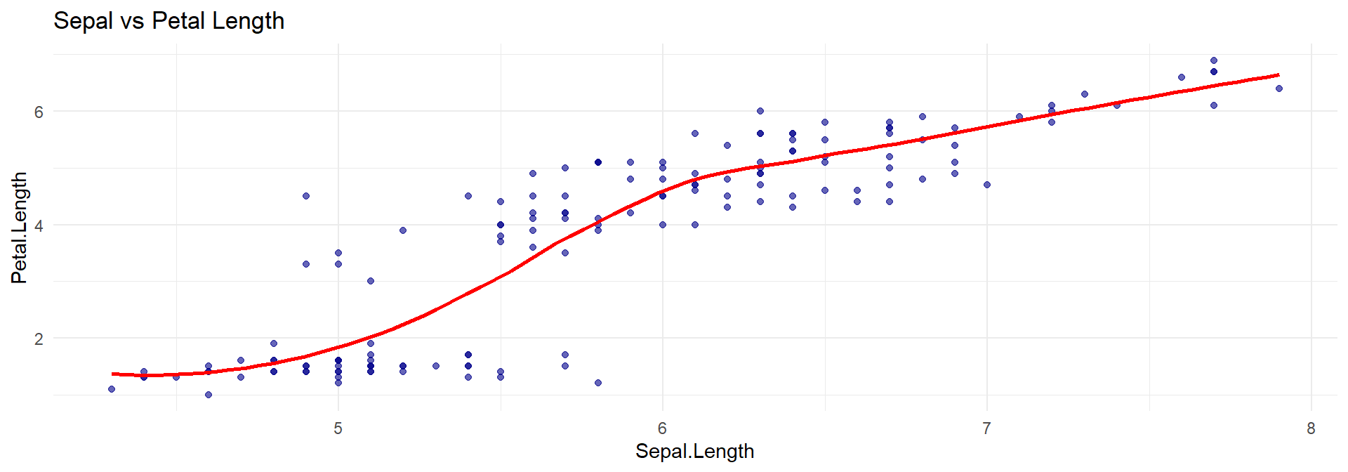
  ggtitle("Petal Length by Species (3 Groups)")

ANOVA Assumptions

Independence → ✔ by design.
Normality within each group

Code

by(iris$Petal.Length, iris$Species, shapiro.test)

iris$Species: setosa

    Shapiro-Wilk normality test

data:  dd[x, ]
W = 0.95498, p-value = 0.05481

------------------------------------------------------------ 
iris$Species: versicolor

    Shapiro-Wilk normality test

data:  dd[x, ]
W = 0.966, p-value = 0.1585

------------------------------------------------------------ 
iris$Species: virginica

    Shapiro-Wilk normality test

data:  dd[x, ]
W = 0.96219, p-value = 0.1098

If some species have p < 0.05, normality is doubtful for those groups.

Homogeneity of variances (Levene)

Code

leveneTest(Petal.Length ~ Species, data = iris)

Levene's Test for Homogeneity of Variance (center = median)
       Df F value    Pr(>F)    
group   2   19.48 3.129e-08 ***
      147                      
---
Signif. codes:  0 '***' 0.001 '**' 0.01 '*' 0.05 '.' 0.1 ' ' 1

If p < 0.05, variances differ across species.

If either normality or variance equality fails → cannot trust ANOVA F-test.

Parametric ANOVA

Code

summary(aov(Petal.Length ~ Species, data = iris))

             Df Sum Sq Mean Sq F value Pr(>F)    
Species       2  437.1  218.55    1180 <2e-16 ***
Residuals   147   27.2    0.19                   
---
Signif. codes:  0 '***' 0.001 '**' 0.01 '*' 0.05 '.' 0.1 ' ' 1

In the ANOVA table, check the row for Species: Pr(>F) is the p-value for group differences.

Non-parametric alternative

Kruskal–Wallis Test

Code

kruskal.test(Petal.Length ~ Species, data = iris)


    Kruskal-Wallis rank sum test

data:  Petal.Length by Species
Kruskal-Wallis chi-squared = 130.41, df = 2, p-value < 2.2e-16

Kruskal–Wallis p-value tests whether at least one group tends to have higher ranks than the others.

If significant → perform post-hoc Dunn tests.

Code

if (!requireNamespace("FSA", quietly = TRUE)) {
  cat("Package 'FSA' not installed; skipping Dunn post-hoc tests. Install with install.packages('FSA').\n")
} else {
  library(FSA)
  dunnTest(Petal.Length ~ Species, data = iris, method = "bonferroni")
}

              Comparison          Z      P.unadj        P.adj
1    setosa - versicolor  -5.862997 4.545875e-09 1.363763e-08
2     setosa - virginica -11.418385 3.384664e-30 1.015399e-29
3 versicolor - virginica  -5.555388 2.769957e-08 8.309872e-08

Post-hoc Dunn tests (when available) show which pairs differ; use adjusted p-values to report significant pairs. If skipped, you can still report the Kruskal–Wallis result and show group medians/IQRs.

Example output and interpretation (R)

Code

aov_res <- aov(Petal.Length ~ Species, data = iris)
kw_res  <- kruskal.test(Petal.Length ~ Species, data = iris)

summary(aov_res)

             Df Sum Sq Mean Sq F value Pr(>F)    
Species       2  437.1  218.55    1180 <2e-16 ***
Residuals   147   27.2    0.19                   
---
Signif. codes:  0 '***' 0.001 '**' 0.01 '*' 0.05 '.' 0.1 ' ' 1

Code

kw_res


    Kruskal-Wallis rank sum test

data:  Petal.Length by Species
Kruskal-Wallis chi-squared = 130.41, df = 2, p-value < 2.2e-16

Code

# Extract and print concise p-values for the slide
s <- summary(aov_res)[[1]]
aov_p <- s[["Pr(>F)"]][1]

Interpretation: With skew/outliers or non-normality, rely on Kruskal–Wallis. If significant, follow with pairwise comparisons (e.g., Dunn tests) and report which species differ.

Correlation Using iris

Goal

Assess the relationship between Sepal.Length and Petal.Length.

Visualise

Code

ggplot(iris, aes(x = Sepal.Length, y = Petal.Length)) +
  geom_point(alpha = 0.6, color = "darkblue") +
  geom_smooth(method = "loess", color = "red", se = FALSE) +
  theme_minimal() +
  ggtitle("Sepal vs Petal Length")

Parametric Correlation (Pearson) Assumptions

Linearity
- The relationship should be a straight line.
Normality
- Both variables should be normally distributed.

Code

shapiro.test(iris$Sepal.Length)


    Shapiro-Wilk normality test

data:  iris$Sepal.Length
W = 0.97609, p-value = 0.01018

Code

shapiro.test(iris$Petal.Length)


    Shapiro-Wilk normality test

data:  iris$Petal.Length
W = 0.87627, p-value = 7.412e-10

If p < 0.05, normality assumption is violated.

Parametric test (Pearson)

Code

cor.test(iris$Sepal.Length, iris$Petal.Length, method = "pearson")


    Pearson's product-moment correlation

data:  iris$Sepal.Length and iris$Petal.Length
t = 21.646, df = 148, p-value < 2.2e-16
alternative hypothesis: true correlation is not equal to 0
95 percent confidence interval:
 0.8270363 0.9055080
sample estimates:
      cor 
0.8717538

Tests for linear correlation.

Non-parametric alternative (if assumptions break)

Spearman’s Rank Correlation

Code

cor.test(iris$Sepal.Length, iris$Petal.Length, method = "spearman")


    Spearman's rank correlation rho

data:  iris$Sepal.Length and iris$Petal.Length
S = 66429, p-value < 2.2e-16
alternative hypothesis: true rho is not equal to 0
sample estimates:
      rho 
0.8818981

Uses ranks; tests for monotonic relationship (doesn’t have to be a straight line, just consistently increasing or decreasing).

Kendall’s Tau

Code

cor.test(iris$Sepal.Length, iris$Petal.Length, method = "kendall")


    Kendall's rank correlation tau

data:  iris$Sepal.Length and iris$Petal.Length
z = 12.647, p-value < 2.2e-16
alternative hypothesis: true tau is not equal to 0
sample estimates:
      tau 
0.7185159

Better for small samples or many ties.
Interpretation: “There is a strong positive monotonic correlation between sepal length and petal length.”

Summary: Use a non-parametric test when:

Data are clearly non-normal (Shapiro–Wilk fails; Q–Q plots bend strongly).
Variances differ strongly across groups (Levene fails).
Data are ordinal (ranks, Likert scores).
There are outliers that distort means.
Sample size is small, making CLT unreliable.
Group distributions have different shapes, not just shifted means.