Call:
lm(formula = body_mass_g ~ bill_length_mm, data = penguins)

Coefficients:
   (Intercept)  bill_length_mm
362.31 87.42 Linear Regression
C5025HF: concepts and intuition
Harper Adams University
What we’re doing today
By the end, you should be able to:
- Explain what a linear model is (and what “linear” actually means)
- Fit and interpret a simple linear regression in R (
lm()) - Distinguish prediction vs explanation (and the traps in each)
- Check assumptions with diagnostic plots
- Report results in a professional, reproducible way
- Recognise when you need extensions: multiple predictors, interactions, blocks, random intercepts
Setup (R)
We’ll use a small, friendly dataset.
Part A — What is a statistical model?
Definition: statistical model
A statistical model is a simplified mathematical description of a real system.
- It focuses on relationships between variables (and uncertainty),
- not just drawing a curve through points.
Linear vs non-linear (intuition)
A relationship can be:
- linear additive: a fixed change in x gives a fixed change in expected y
- non-linear: diminishing returns, saturation, thresholds, etc.
Linear vs non-linear
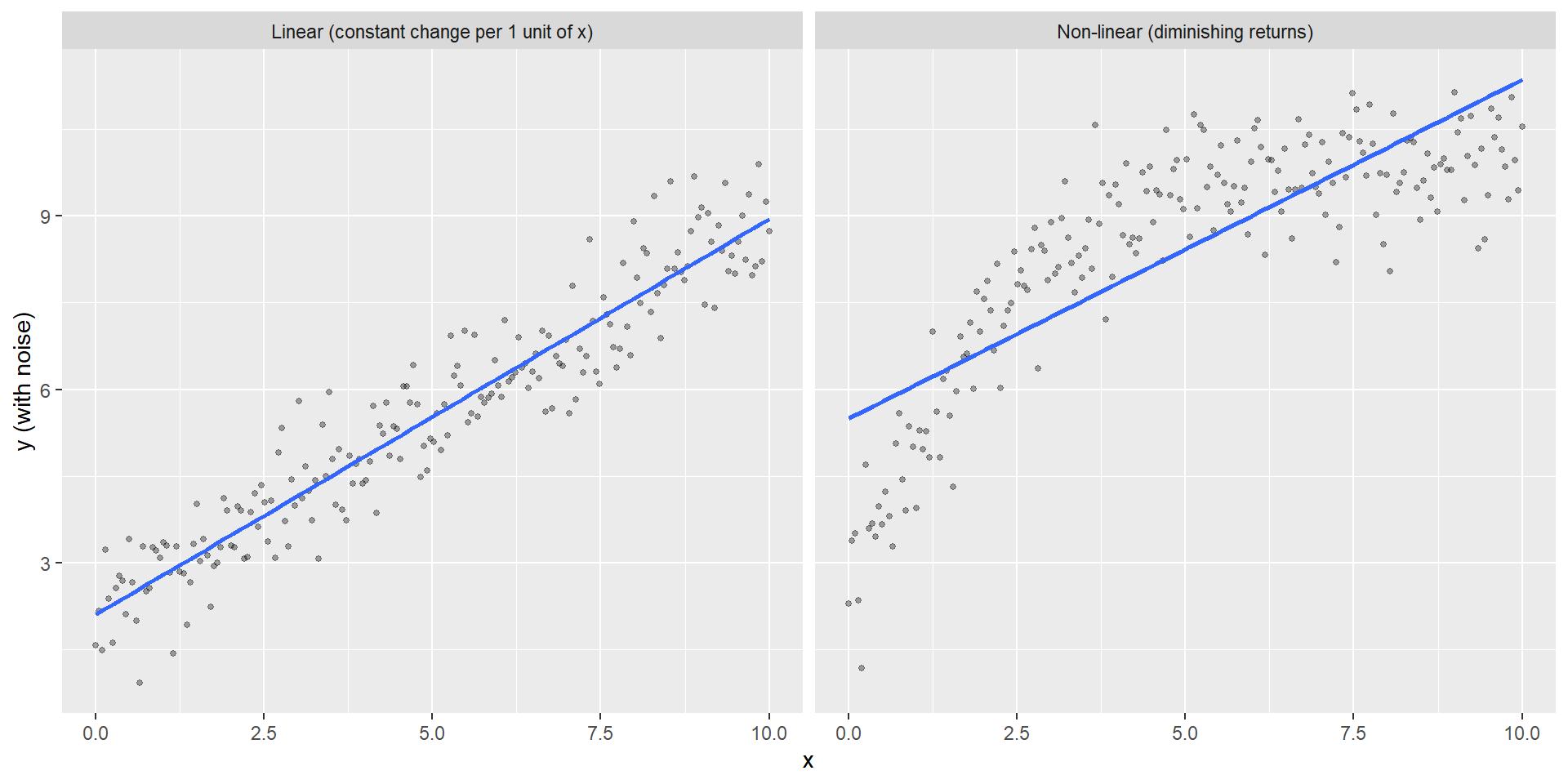
“Linear” means linear in the parameters
A linear model can include transformed predictors:
- ✅
y = β0 + β1 x + β2 x^2 + εis linear in β’s - ✅
y = β0 + β1 log(x) + εis linear in β’s - ❌
y = β0 + exp(β1 x) + εis not linear in β’s
The linear model in matrix form
\[ \mathbf{y} = \mathbf{X}\boldsymbol{\beta} + \boldsymbol{\varepsilon} \]
- y: response/outcome
- X: design matrix (predictors encoded as columns)
- β: coefficients/parameters
- ε: residual error (unexplained part)
What regression is for
Simple regression often answers at least one of:
- Prediction: estimate y at new x
- Explanation: quantify change in y per unit x
- Variance accounting: how much variation in y is associated with x
- Inference: hypothesis tests and confidence intervals
Regression to the mean (intuition)
Regression to the mean happens when you pick people (or things) because they had an extreme result once, then measure them again.
What you see: the extreme scores move closer to average on the second measurement.
Why? Every measurement has some randomness (luck, conditions, mood, error). When you pick “the best” or “the worst” from one measurement, you accidentally pick people who got lucky (or unlucky) that day. Next time, their luck is different—so their score drifts back toward their usual level.
Key examples:
- Students who bombed an exam → tend to do better on a retest (even with no extra study)
- “Rookie of the year” → often has a more normal second season
- Worst-performing stores → often improve next quarter (even with no intervention)
The trap: this looks like improvement (or decline), but it’s just randomness evening out. Nothing actually changed.
Why is it called “regression”?
The connection: linear regression literally models regression to the mean.
History: Francis Galton (1886) studied parent and child heights. He noticed:
- Very tall parents → children are tall, but closer to average height
- Very short parents → children are short, but closer to average height
He called this “regression toward mediocrity” (we now say “regression to the mean”).
Mathematics: When you fit a regression line \(\hat{y} = \alpha + \beta x\), you’re estimating the conditional mean: the average y for a given x.
- If correlation is perfect (\(\rho = 1\)), the line has slope = 1 (no regression to mean)
- If correlation is imperfect (\(\rho < 1\)), the line is flatter than 45°, which means extreme x values predict y values closer to the mean
So: linear regression is the mathematical tool that quantifies how much extreme values regress back toward the mean. The phenomenon gave the method its name!
Caution: correlation ≠ causation
Regression describes association in your dataset.
To talk about causality you need:
- design (randomisation, controls),
- or a strong causal argument (assumptions you can defend).
Part B — Simple linear regression
The simple regression model
\[ y_i = \alpha + \beta x_i + \varepsilon_i,\quad \varepsilon_i \sim \mathcal{N}(0, \sigma^2) \]
- α: intercept (expected y when x = 0)
- β: slope (change in expected y for +1 in x)
- ε: residual (what’s left)
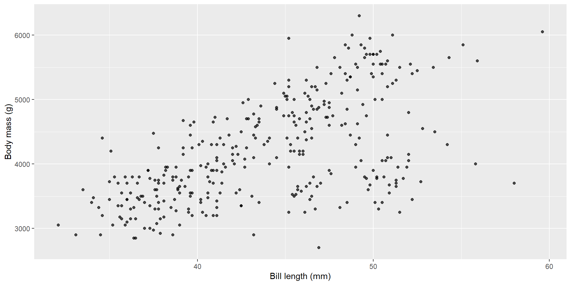
Example: body mass vs bill length
Here’s the relationship we’ll model:
Fit the model with lm()
Add the regression line
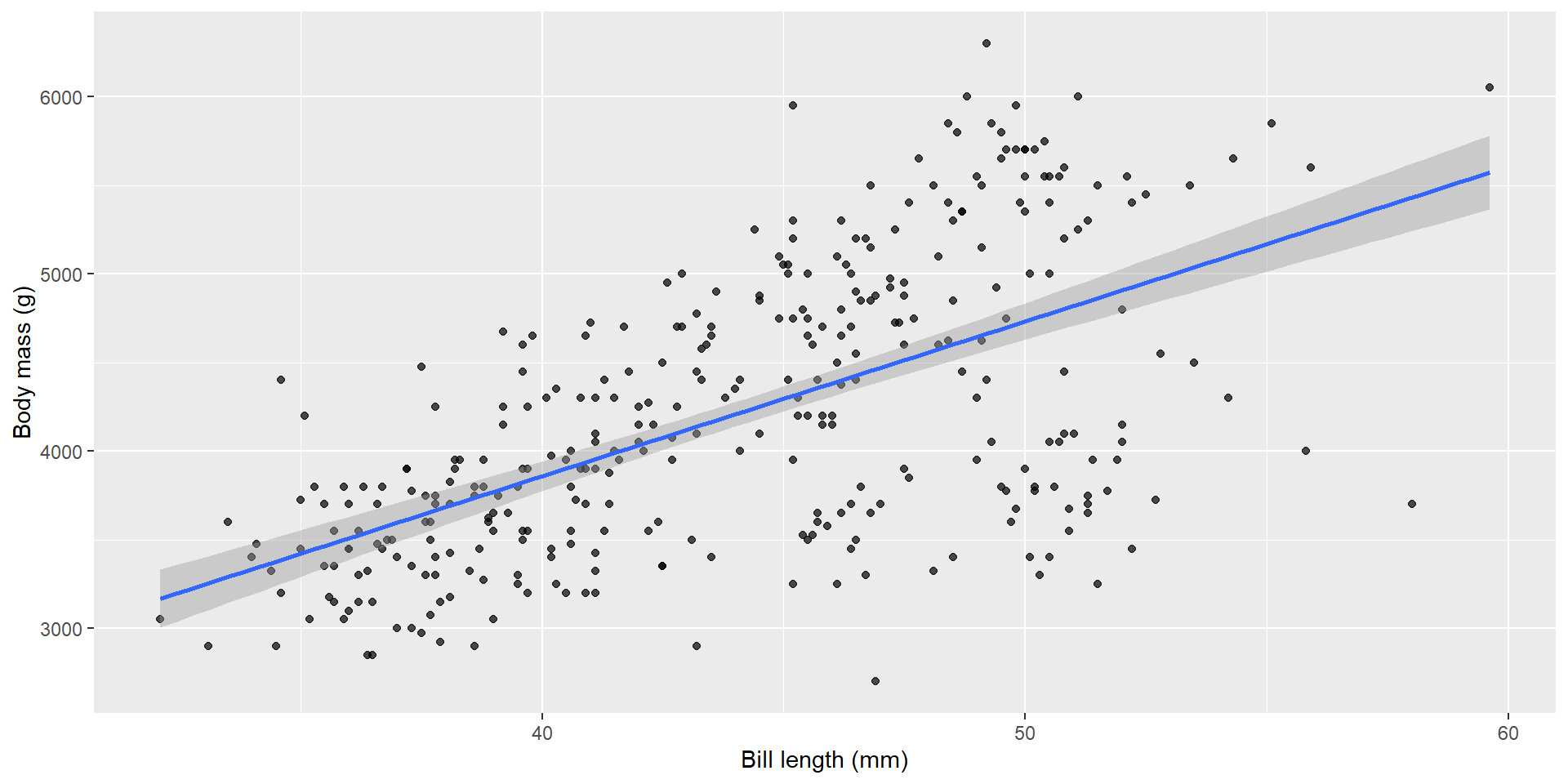
Model coefficients
The fitted regression coefficients with 95% confidence intervals:
| term | estimate | std.error | statistic | p.value | conf.low | conf.high |
|---|---|---|---|---|---|---|
| (Intercept) | 362.31 | 283.35 | 1.28 | 0.2 | -195.02 | 919.64 |
| bill_length_mm | 87.42 | 6.40 | 13.65 | 0.0 | 74.82 | 100.01 |
Interpretation template:
- Slope β: for a 1-unit increase in x, expected y changes by β (holding other predictors constant)
- Intercept α: expected y when x = 0 (sometimes not meaningful!)
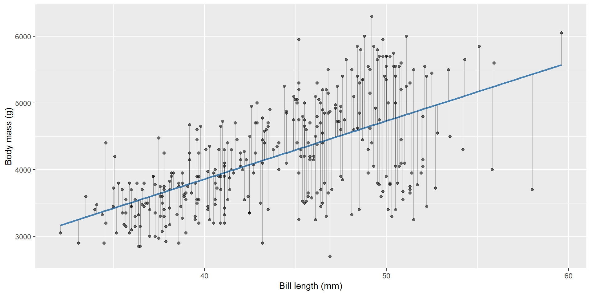
Prediction vs residuals
Two concepts:
- Fitted value: \(\hat{y}_i\) (model’s predicted mean)
- Residual: \(e_i = y_i - \hat{y}_i\)
First few observations with fitted values and residuals:
| Body mass (g) | Bill length (mm) | Fitted | Residual |
|---|---|---|---|
| 3750 | 39.1 | 3780.2 | -30.2 |
| 3800 | 39.5 | 3815.2 | -15.2 |
| 3250 | 40.3 | 3885.1 | -635.1 |
| 3450 | 36.7 | 3570.4 | -120.4 |
| 3650 | 39.3 | 3797.7 | -147.7 |
| 3625 | 38.9 | 3762.8 | -137.8 |
Residuals
Where do the coefficients come from?
Ordinary Least Squares (OLS)
Ordinary least squares chooses alpha, beta to minimise:
\[ \sum_i (y_i - \hat{y}_i)^2 \]
This is the sum of squared residuals.
Why least squares?
- Squaring makes all errors positive
- Larger errors are penalised more heavily
- The mathematics becomes tractable (closed-form solution)
Why ordinary?
Because we assume:
- all observations have equal variance
- all observations are equally reliable
- errors are independent
If these are not true, we move to:
- Weighted least squares (different variances)
- Generalised least squares (correlated errors)
- Mixed models (hierarchical structure)
So “ordinary” = the simplest, default case.
Ordinary least squares (OLS) chooses α, β that minimise:
\[ \sum_i (y_i - \hat{y}_i)^2 \]
This is why you’ll hear “least squares line of best fit”.
R² (variance explained)
How much variation does the model explain?
| R² | Adjusted R² | Residual SD |
|---|---|---|
| 0.354 | 0.352 | 645.433 |
Caution:
- high R² ≠ causal truth
- R² can increase just by adding predictors (use adjusted R², or better, validation)
p-values, confidence intervals, and power
Full model summary:
Call:
lm(formula = body_mass_g ~ bill_length_mm, data = penguins)

Residuals:
     Min       1Q   Median       3Q      Max
-1762.08  -446.98    32.59   462.31  1636.86

Coefficients:
               Estimate Std. Error t value Pr(>|t|)
(Intercept)     362.307    283.345   1.279    0.202
bill_length_mm   87.415      6.402  13.654   <2e-16 ***
---
Signif. codes:  0 '***' 0.001 '**' 0.01 '*' 0.05 '.' 0.1 ' ' 1

Residual standard error: 645.4 on 340 degrees of freedom
Multiple R-squared:  0.3542,    Adjusted R-squared:  0.3523
F-statistic: 186.4 on 1 and 340 DF,  p-value: < 2.2e-16
What is being tested?
For each coefficient \(\beta_j\), the null hypothesis is:
\[ H_0: \beta_j = 0 \]
The test statistic is:
\[ t = \frac{\hat{\beta}_j}{SE(\hat{\beta}_j)} \]
This follows a t-distribution under the model assumptions.
ANOVA view of regression
Analysis of Variance Table

Response: body_mass_g
                Df    Sum Sq  Mean Sq F value    Pr(>F)
bill_length_mm   1  77669072 77669072  186.44 < 2.2e-16 ***
Residuals      340 141638626   416584
---
Signif. codes:  0 '***' 0.001 '**' 0.01 '*' 0.05 '.' 0.1 ' ' 1
ANOVA partitions variance into:
- Model (Regression) sum of squares
- Residual (Error) sum of squares
The F-statistic is:
\[ F = \frac{MS_{model}}{MS_{error}} \]
If this ratio is large, the model explains much more variance than expected by chance.
Confidence intervals
                    2.5 %   97.5 %
(Intercept)    -195.02364 919.6371
bill_length_mm   74.82279 100.0078
A 95% CI is the range of slopes compatible with the data under the model.
Interpreting the regression table
The coefficient table shows estimates, standard errors, t-statistics, and p-values:
| Estimate | Std. Error | t value | Pr(>|t|) | |
|---|---|---|---|---|
| (Intercept) | 362.307 | 283.345 | 1.279 | 0.202 |
| bill_length_mm | 87.415 | 6.402 | 13.654 | 0.000 |
Typical output:
| Term | Estimate | Std. Error | t value | Pr(> |
|---|---|---|---|---|
| (Intercept) | alpha | SE(alpha) | t | p |
| x | beta | SE(beta) | t | p |
How to read this
- Estimate: the fitted coefficient (alpha or beta)
- Std. Error: uncertainty in that estimate
- t value: Estimate / Std. Error
- Pr(>|t|): p-value for H0: coefficient = 0
Intercept
The intercept is the expected value of y when all predictors = 0.
- Sometimes meaningful (e.g. baseline control)
- Often meaningless (e.g. bill length = 0 mm is impossible)
Slope (beta)
The slope is the expected change in y per 1-unit increase in x, holding other predictors constant.
Units always matter:
g per mm, kg per ha, t per °C, etc.
With factors
Call:
lm(formula = body_mass_g ~ species, data = penguins)

Residuals:
     Min       1Q   Median       3Q      Max
-1126.02  -333.09   -33.09   316.91  1223.98

Coefficients:
                 Estimate Std. Error t value Pr(>|t|)
(Intercept)       3700.66      37.62   98.37   <2e-16 ***
speciesChinstrap    32.43      67.51    0.48    0.631
speciesGentoo     1375.35      56.15   24.50   <2e-16 ***
---
Signif. codes:  0 '***' 0.001 '**' 0.01 '*' 0.05 '.' 0.1 ' ' 1

Residual standard error: 462.3 on 339 degrees of freedom
Multiple R-squared:  0.6697,    Adjusted R-squared:  0.6677
F-statistic: 343.6 on 2 and 339 DF,  p-value: < 2.2e-16
Here:
- One level is the reference (baseline)
- Other coefficients are differences from that reference
Example interpretation:
- (Intercept) = mean of reference species
- speciesChinstrap = difference between Chinstrap and reference
With interactions
Model with interaction term:
Call:
lm(formula = body_mass_g ~ bill_length_mm * species, data = penguins)

Residuals:
    Min      1Q  Median      3Q     Max
-918.76 -245.89   -8.65  238.44 1126.27

Coefficients:
                                Estimate Std. Error t value Pr(>|t|)
(Intercept)                        34.88     443.18   0.079    0.937
bill_length_mm                     94.50      11.40   8.291 2.73e-15 ***
speciesChinstrap                  811.26     799.81   1.014    0.311
speciesGentoo                    -158.71     683.19  -0.232    0.816
bill_length_mm:speciesChinstrap   -35.38      17.75  -1.994    0.047 *
bill_length_mm:speciesGentoo       14.96      15.79   0.948    0.344
---
Signif. codes:  0 '***' 0.001 '**' 0.01 '*' 0.05 '.' 0.1 ' ' 1

Residual standard error: 371.8 on 336 degrees of freedom
Multiple R-squared:  0.7882,    Adjusted R-squared:  0.7851
F-statistic: 250.1 on 5 and 336 DF,  p-value: < 2.2e-16
Interpretation:
- Main slope = effect in reference species
- Interaction term = change in slope for the other species
- yield ~ variety * fertiliser: how different is the yield for variety A with fertiliser B from yield for variety A with fertiliser A?
The big rule
Every coefficient is a conditional comparison.
It is always interpreted given the other terms in the model are held constant.
Part C — Assumptions and diagnostics
Core assumptions
In practice we check these assumptions about residuals:
- Linearity of mean structure
- Homoscedasticity (constant variance)
- Independence
- Approximate normality of residuals (mainly for small samples)
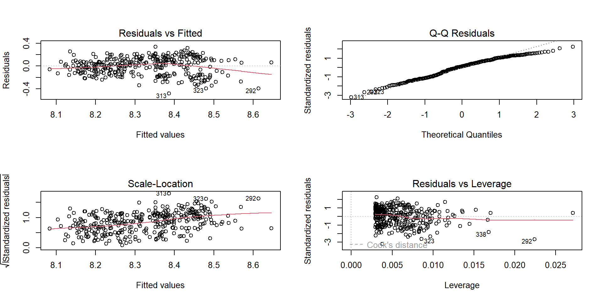
Diagnostic plots in R
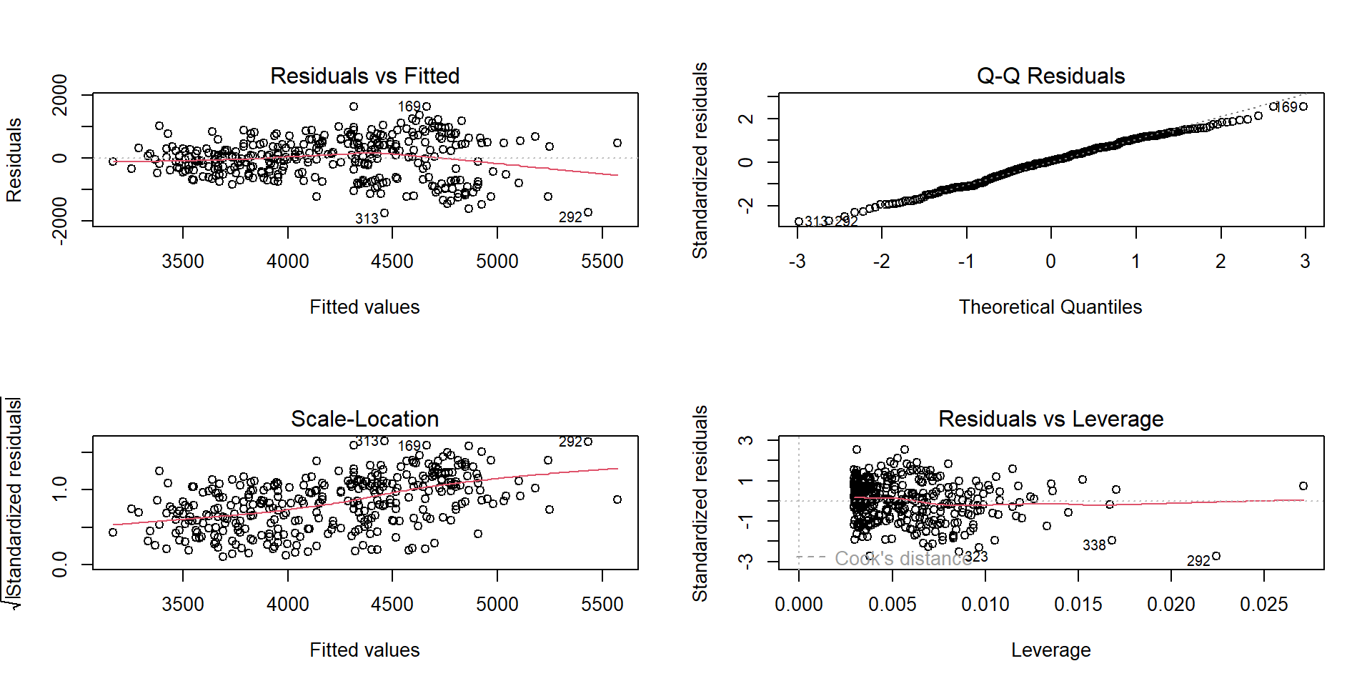
What to look for:
- Residuals vs fitted: pattern? funnel shape?
- Q–Q: strong deviations?
- Scale–Location: heteroscedasticity
- Residuals vs leverage: influential points
Linearity: residual pattern
If you see curvature in residuals vs fitted:
- missing non-linearity (transform x, add polynomial term, or use a better model)
Analysis of Variance Table

Model 1: body_mass_g ~ bill_length_mm
Model 2: body_mass_g ~ poly(bill_length_mm, 2)
  Res.Df       RSS Df Sum of Sq      F   Pr(>F)
1    340 141638626
2    339 138722819  1   2915807 7.1254 0.007966 **
---
Signif. codes:  0 '***' 0.001 '**' 0.01 '*' 0.05 '.' 0.1 ' ' 1
Homoscedasticity: “fan” shape
If residual spread increases with fitted values:
- consider transforming the response (e.g., log)
- consider robust SEs (later modules), or different model family
Independence: design matters
Independence is usually not visible from a single plot.
Breaks happen with:
- repeated measures (same subject multiple times)
- spatial dependence
- time series
If independence is violated, standard errors can be wrong → misleading p-values.
Normality: mostly about small-sample inference
Normal residuals matter most when:
- sample size is small
- you need accurate confidence intervals/tests
With moderate/large samples, regression is often robust, but you still diagnose.
Influential points
Cook’s distance identifies observations that strongly influence the fit. The top 10 most influential observations:
| Body mass (g) | Bill length (mm) | Cook’s D |
|---|---|---|
| 3700 | 58.0 | 0.085 |
| 4000 | 55.8 | 0.032 |
| 3250 | 51.5 | 0.027 |
| 3450 | 52.2 | 0.026 |
| 3725 | 52.7 | 0.020 |
| 6300 | 49.2 | 0.018 |
| 3300 | 50.3 | 0.018 |
| 3400 | 50.5 | 0.017 |
| 3550 | 50.9 | 0.015 |
| 3400 | 50.1 | 0.015 |
Practical fixes (not “magic”)
When assumptions fail:
- rethink the question (is linear regression appropriate?)
- transform variables (log, sqrt)
- add terms (non-linear mean, interactions)
- model grouping (blocks/random intercepts)
- use alternative families (GLMs) or robust methods
Part D — Extensions you’ll meet soon
Multiple regression (main effects)
\[ y = \beta_0 + \beta_1 x_1 + \beta_2 x_2 + \dots + \varepsilon \]
Interpretation: holding other predictors constant.
# A tibble: 3 × 7
  term              estimate std.error statistic  p.value conf.low conf.high
  <chr>                <dbl>     <dbl>     <dbl>    <dbl>    <dbl>     <dbl>
1 (Intercept)       -5737.      308.      -18.6  7.80e-54 -6343.     -5131.
2 bill_length_mm        6.05      5.18      1.17 2.44e- 1    -4.14      16.2
3 flipper_length_mm    48.1       2.01     23.9  7.56e-75    44.2       52.1
Interactions (effect modification)
An interaction means: the effect of x1 depends on x2.
Model with interaction between bill length and species:
| term | estimate | std.error | statistic | p.value |
|---|---|---|---|---|
| (Intercept) | 34.88 | 443.18 | 0.08 | 0.94 |
| bill_length_mm | 94.50 | 11.40 | 8.29 | 0.00 |
| speciesChinstrap | 811.26 | 799.81 | 1.01 | 0.31 |
| speciesGentoo | -158.71 | 683.19 | -0.23 | 0.82 |
| bill_length_mm:speciesChinstrap | -35.38 | 17.75 | -1.99 | 0.05 |
| bill_length_mm:speciesGentoo | 14.96 | 15.79 | 0.95 | 0.34 |
Visualise:
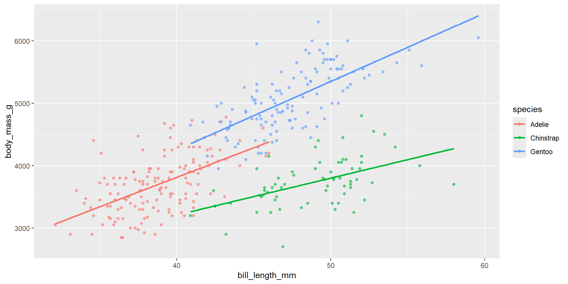
Blocking (fixed effects for batches/sites)
Blocks are nuisance structure you control for.
Adding island as a blocking factor:
| term | estimate | std.error | statistic | p.value | conf.low | conf.high |
|---|---|---|---|---|---|---|
| (Intercept) | 1225.79 | 243.18 | 5.04 | 0 | 747.45 | 1704.13 |
| bill_length_mm | 77.12 | 5.31 | 14.53 | 0 | 66.68 | 87.56 |
| islandDream | -919.07 | 58.62 | -15.68 | 0 | -1034.38 | -803.76 |
| islandTorgersen | -523.29 | 85.55 | -6.12 | 0 | -691.57 | -355.02 |
Random intercepts (preview)
If you have repeated measures, you often want:
\[ y_{ij} = \beta_0 + b_{0i} + \beta_1 x_{ij} + \varepsilon_{ij} \]
- (b_{0i}) is a group-specific intercept deviation (random effect)
In R: lme4::lmer() (covered in mixed models).
Reporting results (what good looks like)
Minimum professional reporting:
- model formula and context (units!)
- coefficient estimate with CI (and p-value if required)
- a goodness-of-fit statement (R², residual SD)
- diagnostics statement (what you checked, any issues)
- a plot (scatter + fitted line; residual checks)
Example sentence:
A linear model indicated that body mass increased with bill length (β = … g/mm, 95% CI …), explaining R² = … of variance; residual plots suggested …