ANOVA - 2
ANOVA with the R Language

ANalysis Of VAriance (ANOVA)
The analysis of variance is not a mathematical theorem, but rather a convenient method of arranging the arithmetic. R. A. Fisher (via Wishart 1934. Sppl. J. Roy. Soc. 1(1):26-61.)
1.1 Objectives
The question of 1-way ANOVA
Data and assumptions
Graphing
Test and alternatives
Practice exercises
ANOVA - When?
anova-able scenarios:
one numeric continuous dependent variable of interest
a factor that contains 2 or more levels, often with a control
When there are just two levels, it’s essentially a t-test
ANOVA - scenarios
overall difference At least one factor mean is different from the rest
Planned comparisons: Targeted orthogonal contrasts
post-hoc tests: compare any factors you want, with some correction.
Partition variation: What’s causing variance in the dependent variable?
Test statistic
- The test statistic for ANOVA is the F ratio
- It is the proportion of variance in the dependent variable between the groups, relative to that within the groups
Data and assumptions
- data example: +experiment in animal genetics, looking at the weight of chickens (8-week old weight in grams), where weight is the continuous dependent variable. The factor is the sire identity; the chicks were sired by one of 5 sires, thus sire is a factor with 5 levels A, B, C, D, and E.
Wide format data
A <- c(687, 691, 793, 675, 700, 753, 704, 717)
B <- c(618, 680, 592, 683, 631, 691, 694, 732)
C <- c(618, 687, 763, 747, 687, 737, 731, 603)
D <- c(600, 657, 669, 606, 718, 693, 669, 648)
E <- c(717, 658, 674, 611, 678, 788, 650, 690)
Long format data (preferred)
- Convert your data to long format (aov in R works with long data)
weight <- c(A,B,C,D,E)
sire <- c(rep("A", 8),
          rep("B", 8),
          rep("C", 8),
          rep("D", 8),
          rep("E", 8) )
new.long<-data.frame(weight, sire)
Assumptions of ANOVA
Gaussian residuals (test graphically)
Homoscedasticity (test graphically, both overall and within factors; residuals versus fitted plot)
Independent observations (assumed)
Formal test of Gaussian residuals
- We can use the shapiro NHST
shapiro.test().
shapiro.test(rstandard(m1))There is no evidence of difference to Gaussian in our residuals for our ANOVA model (Shapiro-Wilk: W = 0.99, n = 40, P = 0.99).
Homoscedasticity check
We will look at the residuals relative to the fitted values.
# Plot for homoscedasticity check
plot(formula = rstandard(m1) ~ fitted(m1),
     ylab = "m1: residuals",
     xlab = "m1: fitted values",
     main = "Spread similar across x?")
abline(h = 0,
       lty = 2, lwd = 2, col = "red")

# Make the mean residual y points (just to check)
y1 <- aggregate(rstandard(m1), by = list(new.long$Sire), FUN = mean)[,2]
# Make the x unique fitted values (just to check)
x1 <- unique(round(fitted(m1), 6))

points(x = x1, y = y1,
       pch = 16, cex = 1.2, col = "blue")
Bartlett test for equal variances between groups
bartlett.test(): do groups have signif different variances?- significant differences = homoskedasticity violated
bartlett.test(formula = weight~sire, data = new.long)We find no evidence that variance in offspring weight differs between sires (Bartlett test: K-sqared = 1.69, df = 4, P = 0.79).
Graphing ANOVA
Recommended: Boxplot, with some way to show the central tendency of the data separately for each factor level. For continuous variables, boxplots show this perfectly.
- For count variables, barplots are sometimes used with the height set to the mean, along with some form of error bar.
Graphing ANOVA
boxplot(Weight ~ Sire, data = new.long,
        ylab = "Weight (g)",
        xlab = "Sire",
        main = "Effect of Sire on 8-wk weight",
        cex = 0)

abline(h = mean(new.long$Weight),
       lty = 2, lwd = 2, col = "red") # Mere vanity

points(x = jitter(rep(1:5, each = 8), amount = .1),
       y = new.long$Weight,
       pch = 16, cex = .8, col = "blue") # Mere vanity
ANOVA basic output
- The ANOVA Table”
- There are 2 rows;for the sire effect and the residual
- The test statistic is the F value (1.87)
- The P-value column is named “Pr(>F)” (0.14)
- There are 4 degrees of freedom for the factor
- Residual degrees of freedom is 35
- No sig evidence that sire explains variation in weight
Contrasts and post hoc test
- Let’s say that sire C is our reference level sire
- For now, we’ll use
lm()to compare everything to sire C - you can generate contrasts and make tests using emmeans e.t.c.
- Let’s interpret the coefficients
- What can we notice about the F value and p-value?
Post hoc tests
The phrase post hoc implies an afterthought. Tread carefully
When multiple tests are made on the same data, it increases the chance of discovering a false positive (Type I error)
p-values can be adjusted to keep Type I error chance at 5%.
Bonferroni
- The Bonferroni adjustment of p-values:
- Simply divides the P by the number of post hoc pairwise comparisons, so you end up evaluating at a lower P-value
- It is considered conservative, and there are alternatives.
- alternatives exists e.g. Tukey’s e.t.c.
- With pairwise.t.test(), the output will be a matrix of p-values
Tukey HSD (Honestly Significant Differences)
- The Tukey HSD test is less conservative Bonferroni
- We use the
Tukey.HSD()function to apply it here. - Also note that the p-values tend to be smaller for the exact same comparisons, but there are sill no significant comparisons.
Alternatives amidst assumption violations
In case the assumptions of 1-way ANOVA cannot be met by the data, there are a few options:
- Transformations (
log(),sqrt()e.t.c.) - GLMs
- Non-parameteric tests: a great escape, but tend to have less power
Kruskal-Wallis alternative to the 1-way ANOVA
# Try this:
# ?kruskal.test
kruskal.test(formula = Weight ~ Sire,
data = new.long)- The result is qualitatively the same as that for our 1-way ANOVA test
ANOVA calculation details
# Our data
chicken.wide
ANOVA Equations
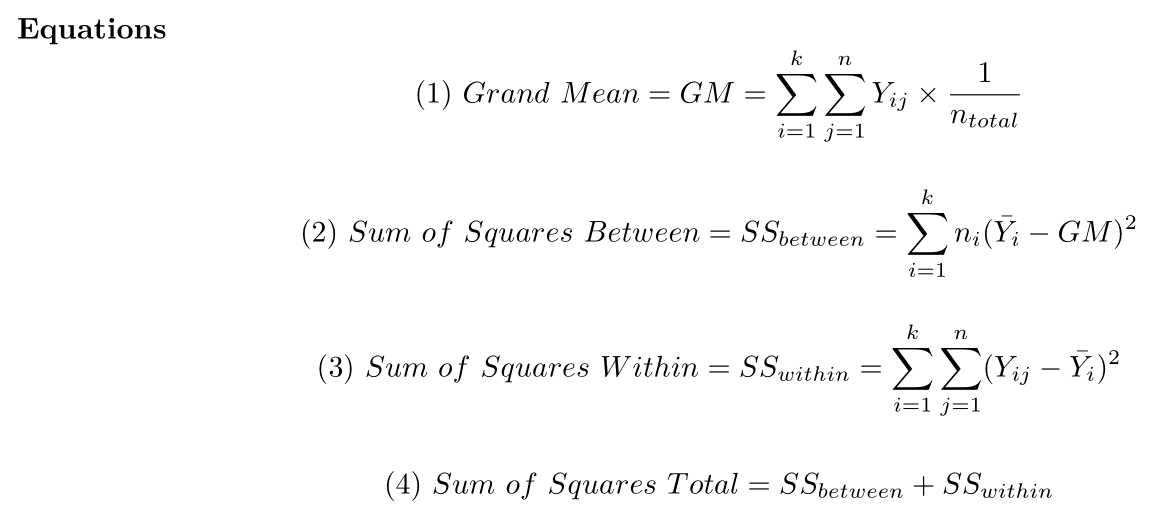 {width = “600px”}
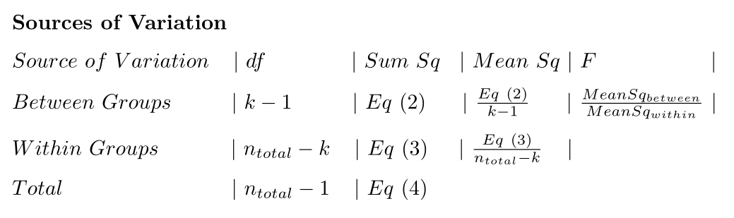
ANOVA Variables
 {width = “400px”}
ANOVA Sources of variation table
 ## Do an ANOVA “by hand” programmatically
- For the ANOVA code in the script, try to follow what is going on in the code
- It is okay if not every detail is clear yet
- Do we get the same answer as aov()?