Regression tutorial

C5025HF: Step-by-step practical guide

Setup

We’ll keep this simple. Just three essential packages:

library(ggplot2)      # for pretty plots
library(dplyr)        # for data wrangling
library(palmerpenguins)  # our dataset

# Load the data and remove rows with missing values
data(penguins)
penguins <- penguins %>%
  filter(!is.na(bill_length_mm), 
         !is.na(body_mass_g), 
         !is.na(species),
         !is.na(flipper_length_mm))

# Take a quick look
head(penguins)

species	island	bill_length_mm	bill_depth_mm	flipper_length_mm	body_mass_g	sex	year
Adelie	Torgersen	39.1	18.7	181	3750	male	2007
Adelie	Torgersen	39.5	17.4	186	3800	female	2007
Adelie	Torgersen	40.3	18.0	195	3250	female	2007
Adelie	Torgersen	36.7	19.3	193	3450	female	2007
Adelie	Torgersen	39.3	20.6	190	3650	male	2007
Adelie	Torgersen	38.9	17.8	181	3625	female	2007

What we’re looking at: Data on 333 penguins from three species. We’ll use their physical measurements to understand regression.

---

Part 1: Simple Linear Regression

The Question: Does bill length predict body mass?

Let’s start with the most basic regression: one predictor, one outcome.

Step 1: Always plot your data first

Never fit a model before looking at your data. Seriously, never.

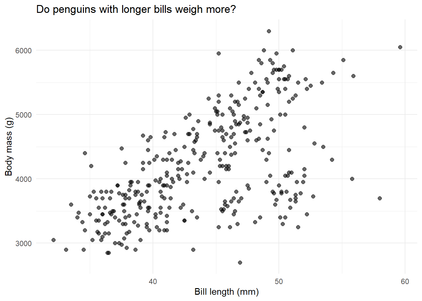
# Create a scatter plot
ggplot(penguins, aes(x = bill_length_mm, y = body_mass_g)) +
  geom_point(alpha = 0.6, size = 2) +
  labs(
    x = "Bill length (mm)",
    y = "Body mass (g)",
    title = "Do penguins with longer bills weigh more?"
  ) +
  theme_minimal()

What do we see? There’s definitely a positive relationship—longer bills tend to go with heavier penguins. But there’s a lot of scatter. Let’s quantify this relationship with regression.

Step 2: Fit the model

The lm() function fits a linear model. The formula y ~ x means “y is predicted by x”.

# Fit the regression: body mass predicted by bill length
model1 <- lm(body_mass_g ~ bill_length_mm, data = penguins)

# The model object is now stored in model1
# Let's see what's inside
class(model1)

[1] "lm"

names(model1)

 [1] "coefficients"  "residuals"     "effects"       "rank"         
 [5] "fitted.values" "assign"        "qr"            "df.residual"  
 [9] "xlevels"       "call"          "terms"         "model"        

What just happened? We created a model object called model1. It’s a list containing everything R calculated: coefficients, residuals, fitted values, and more.

Step 3: Look at the output

# The summary() function shows us the key results
summary(model1)

Call:
lm(formula = body_mass_g ~ bill_length_mm, data = penguins)

Residuals:
     Min       1Q   Median       3Q      Max 
-1762.08  -446.98    32.59   462.31  1636.86 

Coefficients:
               Estimate Std. Error t value Pr(>|t|)    
(Intercept)     362.307    283.345   1.279    0.202    
bill_length_mm   87.415      6.402  13.654   <2e-16 ***
---
Signif. codes:  0 '***' 0.001 '**' 0.01 '*' 0.05 '.' 0.1 ' ' 1

Residual standard error: 645.4 on 340 degrees of freedom
Multiple R-squared:  0.3542,    Adjusted R-squared:  0.3523 
F-statistic: 186.4 on 1 and 340 DF,  p-value: < 2.2e-16

Let’s break this down:

• Coefficients table: Shows our intercept and slope
• Residual standard error: How far off our predictions typically are (645.43g)
• R-squared: Proportion of variance explained (0.35 = 35%)
• F-statistic: Tests if the model is better than just using the mean (it is!)

Step 4: Extract and interpret the coefficients

Instead of just reading the summary, let’s pull out the numbers we need:

# Get the coefficients
coefficients(model1)

   (Intercept) bill_length_mm 
     362.30672       87.41528 

# Or access them directly from the model object
model1$coefficients

   (Intercept) bill_length_mm 
     362.30672       87.41528 

What do these mean?

• Intercept = 362.31: A penguin with 0mm bill length would weigh 362.31g. (Obviously impossible—this is just where the line crosses the y-axis)
• Slope = 87.42: For every 1mm increase in bill length, body mass increases by 87.42 grams on average

Let’s get confidence intervals too:

# 95% confidence intervals for our coefficients
ci1 <- confint(model1)
ci1

                    2.5 %   97.5 %
(Intercept)    -195.02364 919.6371
bill_length_mm   74.82279 100.0078

We’re 95% confident the true slope is between 74.82 and 100.01 grams per mm.

Step 5: Get R-squared

How much of the variation in body mass does bill length explain?

# Extract R-squared from the summary
r2_model1 <- summary(model1)$r.squared
r2_model1

[1] 0.3541557

# For adjusted R-squared
summary(model1)$adj.r.squared

[1] 0.3522562

35% explained. That means bill length accounts for about a third of why some penguins are heavier than others. Not bad, but there’s clearly more to the story.

Step 6: Add the regression line to our plot

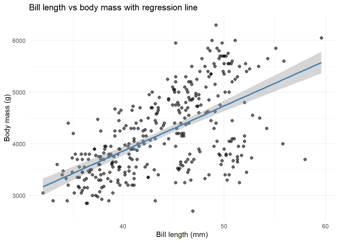
ggplot(penguins, aes(x = bill_length_mm, y = body_mass_g)) +
  geom_point(alpha = 0.6, size = 2) +
  geom_smooth(method = "lm", se = TRUE, color = "steelblue") +
  labs(
    x = "Bill length (mm)",
    y = "Body mass (g)",
    title = "Bill length vs body mass with regression line"
  ) +
  theme_minimal()

The shaded area shows our uncertainty about where the true line is.

Step 7: Understand predictions and residuals

Let’s manually see what the model predicts:

# Get fitted (predicted) values for each penguin
fitted_values <- fitted(model1)

# Get residuals (observed - predicted)
residuals_values <- residuals(model1)

# Look at first 10 penguins
data.frame(
  observed = penguins$body_mass_g[1:10],
  predicted = fitted_values[1:10],
  residual = residuals_values[1:10]
)

observed	predicted	residual
3750	3780.244	-30.24405
3800	3815.210	-15.21017
3250	3885.142	-635.14239
3450	3570.447	-120.44739
3650	3797.727	-147.72711
3625	3762.761	-137.76100
4675	3788.986	886.01442
3475	3343.168	131.83233
4250	4033.748	216.25164
3300	3666.604	-366.60419

What’s a residual? It’s how wrong we were. If a penguin weighs 3750g but we predicted 3600g, the residual is +150g. Positive residuals mean we underestimated; negative means we overestimated.

---

Part 2: Multiple Regression

The Question: Does adding flipper length improve our predictions?

We saw that bill length explains 35% of body mass variation. Can we do better by adding another predictor?

Step 1: Visualize both predictors

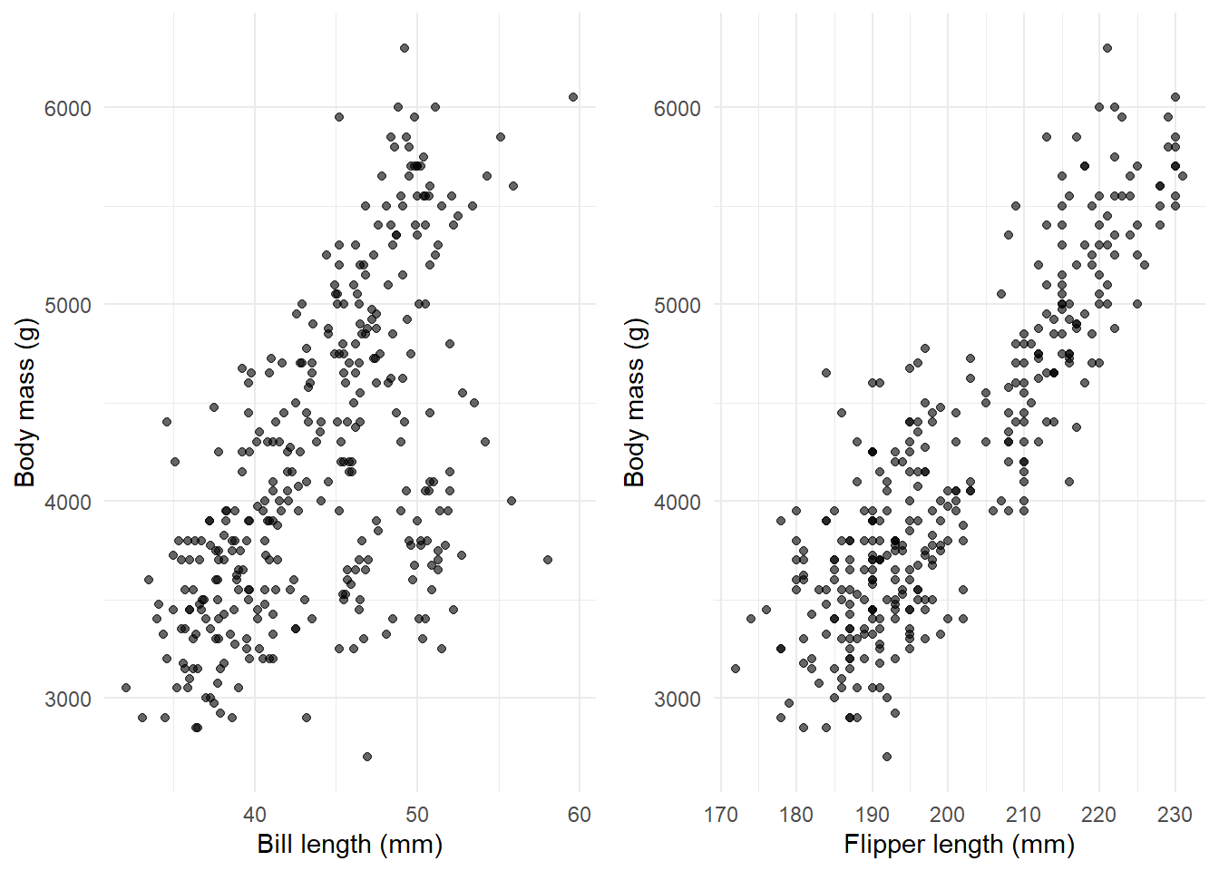
# Create two plots side by side
library(gridExtra)

p1 <- ggplot(penguins, aes(x = bill_length_mm, y = body_mass_g)) +
  geom_point(alpha = 0.6) +
  labs(x = "Bill length (mm)", y = "Body mass (g)") +
  theme_minimal()

p2 <- ggplot(penguins, aes(x = flipper_length_mm, y = body_mass_g)) +
  geom_point(alpha = 0.6) +
  labs(x = "Flipper length (mm)", y = "Body mass (g)") +
  theme_minimal()

grid.arrange(p1, p2, ncol = 2)

Both show positive relationships. Now let’s include both in one model.

Step 2: Fit the multiple regression

The + sign means “include both predictors”:

# Fit model with two predictors
model2 <- lm(body_mass_g ~ bill_length_mm + flipper_length_mm, data = penguins)

summary(model2)

Call:
lm(formula = body_mass_g ~ bill_length_mm + flipper_length_mm, 
    data = penguins)

Residuals:
    Min      1Q  Median      3Q     Max 
-1090.5  -285.7   -32.1   244.2  1287.5 

Coefficients:
                   Estimate Std. Error t value Pr(>|t|)    
(Intercept)       -5736.897    307.959 -18.629   <2e-16 ***
bill_length_mm        6.047      5.180   1.168    0.244    
flipper_length_mm    48.145      2.011  23.939   <2e-16 ***
---
Signif. codes:  0 '***' 0.001 '**' 0.01 '*' 0.05 '.' 0.1 ' ' 1

Residual standard error: 394.1 on 339 degrees of freedom
Multiple R-squared:   0.76, Adjusted R-squared:  0.7585 
F-statistic: 536.6 on 2 and 339 DF,  p-value: < 2.2e-16

Step 3: Interpret the coefficients carefully

This is where multiple regression gets interesting:

coefficients(model2)

      (Intercept)    bill_length_mm flipper_length_mm 
     -5736.897161          6.047488         48.144859 

ci2 <- confint(model2)
ci2

                        2.5 %      97.5 %
(Intercept)       -6342.64860 -5131.14573
bill_length_mm       -4.14117    16.23615
flipper_length_mm    44.18902    52.10069

What do these mean?

• bill_length_mm = 6.05: Holding flipper length constant, a 1mm increase in bill length increases body mass by 6.05g
• flipper_length_mm = 48.14: Holding bill length constant, a 1mm increase in flipper length increases body mass by 48.14g

Wait, what happened? The bill length effect dropped from 87.42g to 6.05g! Why? Because bill length and flipper length are correlated—they both measure “penguin size”. Once we account for flipper length, bill length doesn’t add as much.

Step 4: Compare model fit

Did adding flipper length help?

# Model 1 R-squared
r2_model1

[1] 0.3541557

# Model 2 R-squared  
r2_model2 <- summary(model2)$r.squared
r2_model2

[1] 0.7599577

Huge improvement! We went from 35% to 76% variance explained. Flipper length is clearly an important predictor.

Step 5: Formal model comparison

We can test if model2 is significantly better than model1:

# ANOVA compares nested models
anova(model1, model2)

Res.Df	RSS	Df	Sum of Sq	F	Pr(>F)
340	141638626	NA	NA	NA	NA
339	52643125	1	88995501	573.0943	0

Reading the output: The p-value is tiny (< 0.001), confirming that adding flipper length significantly improves the model.

---

Part 3: Interactions

The Question: Does the bill-length effect differ by species?

Maybe the relationship between bill length and body mass isn’t the same for all three species.

Step 1: Plot by species

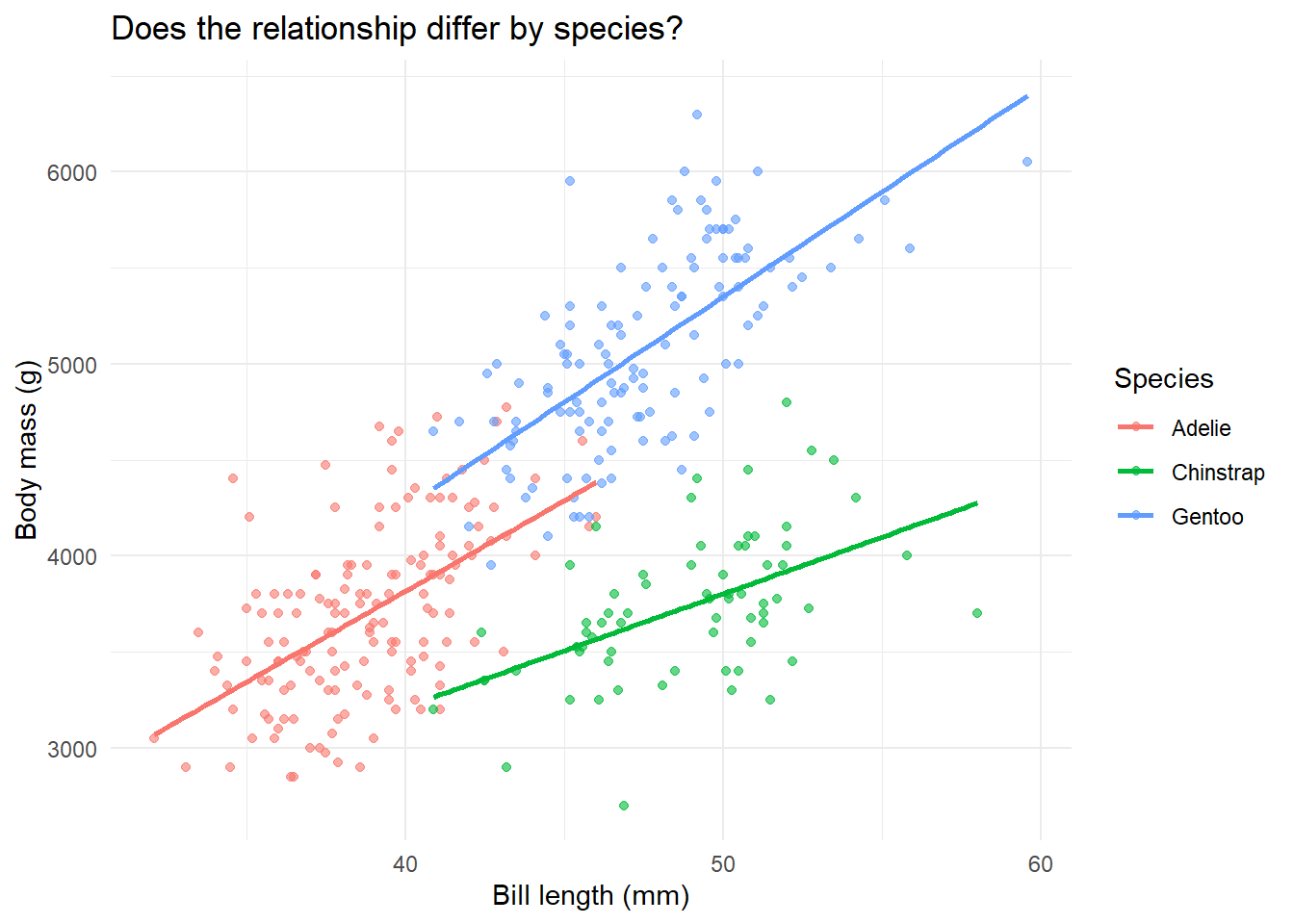
ggplot(penguins, aes(x = bill_length_mm, y = body_mass_g, color = species)) +
  geom_point(alpha = 0.6) +
  geom_smooth(method = "lm", se = FALSE) +
  labs(
    x = "Bill length (mm)",
    y = "Body mass (g)",
    title = "Does the relationship differ by species?",
    color = "Species"
  ) +
  theme_minimal()

What do we see? Three different regression lines with different slopes. Adelie (pink) has a gentler slope than Gentoo (green). This suggests an interaction.

Step 2: Fit the interaction model

The * symbol means “include both main effects AND their interaction”:

# Main effects + interaction
model3 <- lm(body_mass_g ~ bill_length_mm * species, data = penguins)

summary(model3)

Call:
lm(formula = body_mass_g ~ bill_length_mm * species, data = penguins)

Residuals:
    Min      1Q  Median      3Q     Max 
-918.76 -245.89   -8.65  238.44 1126.27 

Coefficients:
                                Estimate Std. Error t value Pr(>|t|)    
(Intercept)                        34.88     443.18   0.079    0.937    
bill_length_mm                     94.50      11.40   8.291 2.73e-15 ***
speciesChinstrap                  811.26     799.81   1.014    0.311    
speciesGentoo                    -158.71     683.19  -0.232    0.816    
bill_length_mm:speciesChinstrap   -35.38      17.75  -1.994    0.047 *  
bill_length_mm:speciesGentoo       14.96      15.79   0.948    0.344    
---
Signif. codes:  0 '***' 0.001 '**' 0.01 '*' 0.05 '.' 0.1 ' ' 1

Residual standard error: 371.8 on 336 degrees of freedom
Multiple R-squared:  0.7882,    Adjusted R-squared:  0.7851 
F-statistic: 250.1 on 5 and 336 DF,  p-value: < 2.2e-16

Step 3: Interpret interaction coefficients

This is the trickiest part of regression. Let’s go slowly:

coefficients(model3)

                    (Intercept)                  bill_length_mm 
                       34.88299                        94.49982 
               speciesChinstrap                   speciesGentoo 
                      811.26034                      -158.71092 
bill_length_mm:speciesChinstrap    bill_length_mm:speciesGentoo 
                      -35.38208                        14.95935 

How to read this:

1. Intercept and bill_length_mm: These apply to the reference species (Adelie, alphabetically first)
2. speciesChinstrap and speciesGentoo: These are adjustments to the intercept for those species
3. bill_length_mm:speciesChinstrap and bill_length_mm:speciesGentoo: These are adjustments to the slope for those species

Species-specific slopes:

# Extract coefficients
coef3 <- coefficients(model3)

# Calculate species-specific slopes
slope_adelie <- coef3["bill_length_mm"]
slope_chinstrap <- coef3["bill_length_mm"] + coef3["bill_length_mm:speciesChinstrap"]
slope_gentoo <- coef3["bill_length_mm"] + coef3["bill_length_mm:speciesGentoo"]

# Display them
data.frame(
  Species = c("Adelie", "Chinstrap", "Gentoo"),
  Slope = round(c(slope_adelie, slope_chinstrap, slope_gentoo), 2)
)

Species	Slope
Adelie	94.50
Chinstrap	59.12
Gentoo	109.46

• Adelie: 94.5 g/mm
• Chinstrap: 59.12 g/mm
  
• Gentoo: 109.46 g/mm

Step 4: Do we need the interaction?

Test if the interaction terms improve the model:

# Model without interaction
model3_simple <- lm(body_mass_g ~ bill_length_mm + species, data = penguins)

# Compare
anova_comparison <- anova(model3_simple, model3)
anova_comparison

Res.Df	RSS	Df	Sum of Sq	F	Pr(>F)
338	47613707	NA	NA	NA	NA
336	46447006	2	1166702	4.21999	0.0154854

The p-value is 0.015. Since this is less than 0.05, the interaction is statistically significant. The slopes really do differ across species. We should keep the interaction in the model!

---

Part 4: ANOVA is Just Regression

The Big Reveal: ANOVA = Regression with categorical predictors

This blows people’s minds every time. Let’s prove it.

Traditional ANOVA approach

Do the three species have different average body masses?

# Fit ANOVA
aov_model <- aov(body_mass_g ~ species, data = penguins)
aov_summary <- summary(aov_model)
aov_summary

             Df    Sum Sq  Mean Sq F value Pr(>F)    
species       2 146864214 73432107   343.6 <2e-16 ***
Residuals   339  72443483   213698                   
---
Signif. codes:  0 '***' 0.001 '**' 0.01 '*' 0.05 '.' 0.1 ' ' 1

ANOVA says: F = 343.63, p < 0.001. Species significantly affect body mass.

Regression approach

Now let’s use lm() with a categorical predictor:

# Fit regression with species as predictor
lm_model <- lm(body_mass_g ~ species, data = penguins)
lm_summary <- summary(lm_model)
lm_summary

Call:
lm(formula = body_mass_g ~ species, data = penguins)

Residuals:
     Min       1Q   Median       3Q      Max 
-1126.02  -333.09   -33.09   316.91  1223.98 

Coefficients:
                 Estimate Std. Error t value Pr(>|t|)    
(Intercept)       3700.66      37.62   98.37   <2e-16 ***
speciesChinstrap    32.43      67.51    0.48    0.631    
speciesGentoo     1375.35      56.15   24.50   <2e-16 ***
---
Signif. codes:  0 '***' 0.001 '**' 0.01 '*' 0.05 '.' 0.1 ' ' 1

Residual standard error: 462.3 on 339 degrees of freedom
Multiple R-squared:  0.6697,    Adjusted R-squared:  0.6677 
F-statistic: 343.6 on 2 and 339 DF,  p-value: < 2.2e-16

Notice the bottom line: F-statistic: 343.63, p < 0.001

They’re identical!

# Get ANOVA table from the lm model
anova(lm_model)

	Df	Sum Sq	Mean Sq	F value	Pr(>F)
species	2	146864214	73432107.1	343.6263	0
Residuals	339	72443483	213697.6	NA	NA

Same F-statistic, same p-value, same conclusion. ANOVA is just regression where the predictor is categorical instead of continuous.

What do the regression coefficients mean?

coef_lm <- coefficients(lm_model)
coef_lm

     (Intercept) speciesChinstrap    speciesGentoo 
      3700.66225         32.42598       1375.35401 

• Intercept (3700.66): Mean body mass for Adelie (the reference group)
• speciesChinstrap (32.43): Chinstrap penguins weigh 32.43g less than Adelie, on average
• speciesGentoo (1375.35): Gentoo penguins weigh 1375.35g more than Adelie, on average

Let’s verify this by calculating group means directly:

# Calculate means by species
species_means <- penguins %>%
  group_by(species) %>%
  summarise(mean_mass = mean(body_mass_g))
species_means

species	mean_mass
Adelie	3700.662
Chinstrap	3733.088
Gentoo	5076.016

• Adelie: 3700.66g (= intercept)
• Chinstrap: 3733.09g = 3700.66 + 32.43 ✓
• Gentoo: 5076.02g = 3700.66 + 1375.35 ✓

The regression coefficients directly tell us group differences!

---

Part 5: Checking Your Model (Diagnostics)

Why diagnostics matter

Regression makes assumptions. If those assumptions are violated, your p-values and confidence intervals are unreliable. We need to check:

1. Linearity: Is the relationship actually linear?
2. Homoscedasticity: Is the variance constant?
3. Normality: Are residuals roughly normal?
4. Independence: Are observations independent? (Check by study design)

The four diagnostic plots

R gives us four helpful plots. Let’s use model2 (body mass ~ bill length + flipper length):

# Create all four diagnostic plots
par(mfrow = c(2, 2))  # 2x2 grid of plots
plot(model2)

par(mfrow = c(1, 1))  # reset to single plot

How to read each plot

Plot 1: Residuals vs Fitted

• What to look for: Random scatter around the horizontal line at zero
• Red flag: A pattern (curve, U-shape) means the relationship isn’t linear
• Red flag: A funnel shape (wider on one side) means variance isn’t constant

Plot 2: Normal Q-Q

• What to look for: Points following the diagonal line
• Red flag: Points curving away from the line means residuals aren’t normal
• Note: Small deviations at the ends are usually okay

Plot 3: Scale-Location

• What to look for: Random scatter, roughly flat red line
• Red flag: Red line sloping up means variance increases with fitted values
• This checks: Homoscedasticity (constant variance)

Plot 4: Residuals vs Leverage

• What to look for: All points inside the dashed lines (Cook’s distance)
• Red flag: Points outside the dashed lines have high influence
• What it means: These observations strongly affect the regression line

What does model2 look like?

Looking at our four plots:

• Residuals vs Fitted: Pretty random, no strong pattern
• Q-Q plot: Points mostly follow the line; residuals are roughly normal
• Scale-Location: Fairly flat; variance looks constant
• Residuals vs Leverage: No points way outside; no highly influential observations

Verdict: This model looks good! Assumptions are reasonably met.

When things go wrong: An example

Let’s see what bad diagnostics look like. We’ll fit a model that doesn’t account for species:

# Deliberately ignoring species
bad_model <- lm(body_mass_g ~ bill_length_mm, data = penguins)

par(mfrow = c(2, 2))
plot(bad_model)

par(mfrow = c(1, 1))

What’s wrong here?

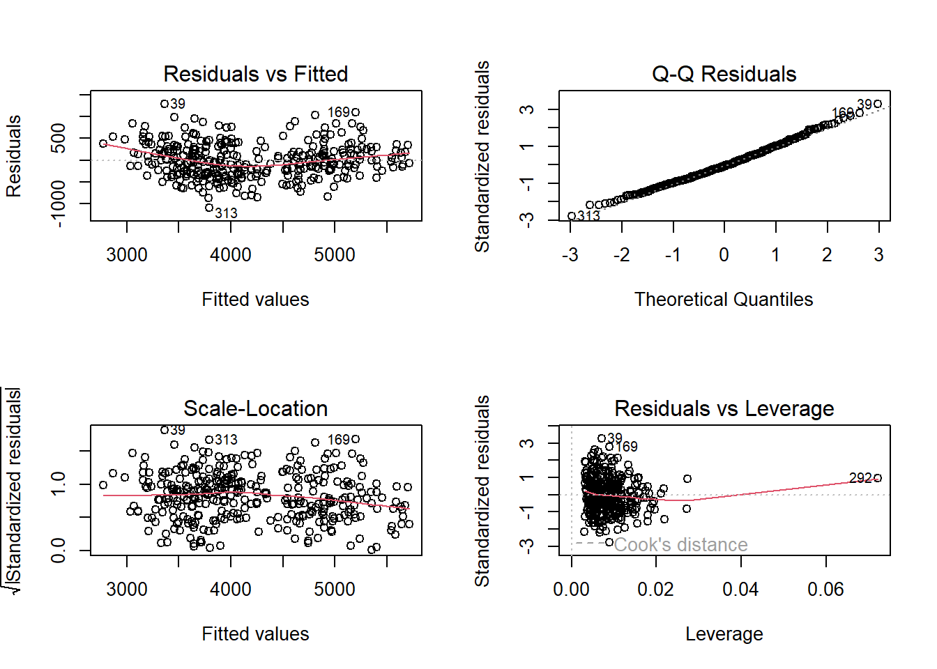
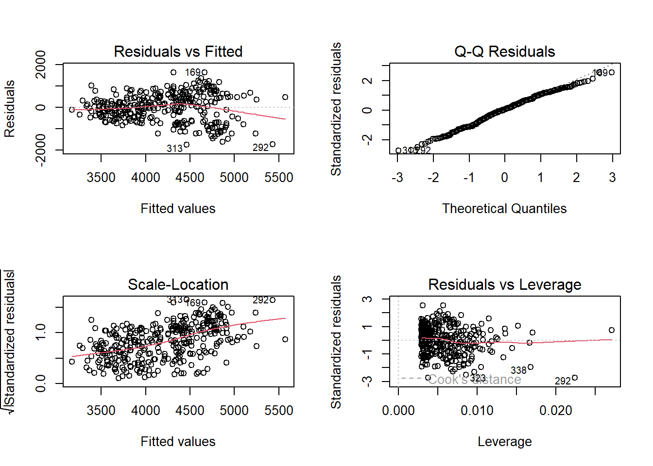
• Residuals vs Fitted: You can see some pattern/grouping—we’re missing an important predictor (species)
• Q-Q plot: Tails deviate more from the line
• This shows why model2 (which includes flipper length) is better

---

Summary: The Essential R Commands

Here’s everything you need to know:

# Fit a model
model <- lm(y ~ x, data = mydata)                    # simple regression
model <- lm(y ~ x1 + x2, data = mydata)              # multiple regression
model <- lm(y ~ x1 * x2, data = mydata)              # with interaction

# Look at results
summary(model)                # full output
coefficients(model)           # just the coefficients
confint(model)               # confidence intervals
anova(model)                 # ANOVA table

# Extract components
model$coefficients           # coefficients
fitted(model)               # predicted values
residuals(model)            # residuals
summary(model)$r.squared    # R-squared

# Compare models
anova(model1, model2)       # test if model2 is better

# Diagnostics
plot(model)                 # creates 4 diagnostic plots

---

Practice Exercises

Try these yourself:

1. Fit a simple regression predicting body_mass_g from flipper_length_mm. What’s the slope? Interpret it in plain English.

2. Add bill_length_mm to create a multiple regression. How did the flipper length coefficient change?

3. Fit separate regressions for each species (use filter()). Do Adelie, Chinstrap, and Gentoo have different slopes?

4. Use lm() to test if body mass differs between male and female penguins. Then verify your answer using t.test().

5. Check the diagnostics for your models. Do any assumptions look violated?

---

What You’ve Learned

• How to fit linear models with lm()
• How to extract and interpret coefficients
• The difference between simple and multiple regression
• What interactions mean and how to test them
• That ANOVA is secretly just regression
• How to check if your model assumptions are met

Most importantly: You learned to interrogate model objects directly using base R, not relying on fancy packages. This is how you really understand what’s going on under the hood.

Now go practice with your own data!